Tutorials


QGIS Tutorial
GeoHealth publications
		4800755


		1
		apa
		50
		date
		desc
		year


		1
		1


        523
		https://geohealthresearch.org/wp-content/plugins/zotpress/


				%7B%22status%22%3A%22success%22%2C%22updateneeded%22%3Afalse%2C%22instance%22%3Afalse%2C%22meta%22%3A%7B%22request_last%22%3A50%2C%22request_next%22%3A50%2C%22used_cache%22%3Atrue%7D%2C%22data%22%3A%5B%7B%22key%22%3A%22S9DVYJ6T%22%2C%22library%22%3A%7B%22id%22%3A4800755%7D%2C%22meta%22%3A%7B%22creatorSummary%22%3A%22Herbreteau%20and%20Picardeau%22%2C%22parsedDate%22%3A%222026-04-22%22%2C%22numChildren%22%3A0%7D%2C%22bib%22%3A%22%26lt%3Bdiv%20class%3D%26quot%3Bcsl-bib-body%26quot%3B%20style%3D%26quot%3Bline-height%3A%202%3B%20padding-left%3A%201em%3B%20text-indent%3A-1em%3B%26quot%3B%26gt%3B%5Cn%20%20%26lt%3Bdiv%20class%3D%26quot%3Bcsl-entry%26quot%3B%26gt%3BHerbreteau%2C%20V.%2C%20%26amp%3B%20Picardeau%2C%20M.%20%282026%29.%20Climate%20Change%20and%20Leptospirosis%3A%20A%20growing%20Environmental%20and%20Zoonotic%20Threat.%20%26lt%3Bi%26gt%3BmicroLife%26lt%3B%5C%2Fi%26gt%3B%2C%20uqag015.%20%26lt%3Ba%20class%3D%26%23039%3Bzp-DOIURL%26%23039%3B%20target%3D%26%23039%3B_blank%26%23039%3B%20href%3D%26%23039%3Bhttps%3A%5C%2F%5C%2Fdoi.org%5C%2F10.1093%5C%2Ffemsml%5C%2Fuqag015%26%23039%3B%26gt%3Bhttps%3A%5C%2F%5C%2Fdoi.org%5C%2F10.1093%5C%2Ffemsml%5C%2Fuqag015%26lt%3B%5C%2Fa%26gt%3B%20%26lt%3Ba%20title%3D%26%23039%3BCite%20in%20RIS%20Format%26%23039%3B%20class%3D%26%23039%3Bzp-CiteRIS%26%23039%3B%20data-zp-cite%3D%26%23039%3Bapi_user_id%3D4800755%26amp%3Bitem_key%3DS9DVYJ6T%26%23039%3B%20href%3D%26%23039%3Bjavascript%3Avoid%280%29%3B%26%23039%3B%26gt%3BCite%26lt%3B%5C%2Fa%26gt%3B%20%26lt%3B%5C%2Fdiv%26gt%3B%5Cn%26lt%3B%5C%2Fdiv%26gt%3B%22%2C%22data%22%3A%7B%22itemType%22%3A%22journalArticle%22%2C%22title%22%3A%22Climate%20Change%20and%20Leptospirosis%3A%20A%20growing%20Environmental%20and%20Zoonotic%20Threat%22%2C%22creators%22%3A%5B%7B%22creatorType%22%3A%22author%22%2C%22firstName%22%3A%22Vincent%22%2C%22lastName%22%3A%22Herbreteau%22%7D%2C%7B%22creatorType%22%3A%22author%22%2C%22firstName%22%3A%22Mathieu%22%2C%22lastName%22%3A%22Picardeau%22%7D%5D%2C%22abstractNote%22%3A%22Abstract%5Cn%20%20%20%20%20%20%20%20%20%20%20%20Climate%20change%20is%20increasingly%20recognized%20as%20a%20key%20driver%20in%20the%20emergence%20and%20re-emergence%20of%20infectious%20diseases%2C%20including%20leptospirosis%2C%20a%20globally%20distributed%20bacterial%20zoonosis.%20The%20bacterial%20agents%20of%20leptospirosis%20infect%20humans%20through%20contact%20with%20soil%20or%20water%20contaminated%20by%20the%20urine%20of%20animal%20reservoirs.%20As%20a%20primarily%20waterborne%20disease%2C%20leptospirosis%20is%20strongly%20influenced%20by%20climatic%20conditions%2C%20including%20rainfall%2C%20flooding%2C%20and%20extreme%20events%20such%20as%20hurricanes%20and%20cyclones.%20Here%2C%20we%20present%20current%20knowledge%20on%20the%20links%20between%20climate%20change%20and%20leptospirosis%2C%20as%20well%20as%20perspectives%20on%20effective%20strategies%20to%20combat%20this%20disease%2C%20which%20disproportionately%20affects%20the%20poorest%20populations.%22%2C%22date%22%3A%222026-04-22%22%2C%22section%22%3A%22%22%2C%22partNumber%22%3A%22%22%2C%22partTitle%22%3A%22%22%2C%22DOI%22%3A%2210.1093%5C%2Ffemsml%5C%2Fuqag015%22%2C%22citationKey%22%3A%22%22%2C%22url%22%3A%22https%3A%5C%2F%5C%2Facademic.oup.com%5C%2Fmicrolife%5C%2Fadvance-article%5C%2Fdoi%5C%2F10.1093%5C%2Ffemsml%5C%2Fuqag015%5C%2F8660968%22%2C%22PMID%22%3A%22%22%2C%22PMCID%22%3A%22%22%2C%22ISSN%22%3A%222633-6693%22%2C%22language%22%3A%22en%22%2C%22collections%22%3A%5B%5D%2C%22dateModified%22%3A%222026-04-23T03%3A31%3A02Z%22%7D%7D%2C%7B%22key%22%3A%22CE7R7FK5%22%2C%22library%22%3A%7B%22id%22%3A4800755%7D%2C%22meta%22%3A%7B%22creatorSummary%22%3A%22Artadji%20et%20al.%22%2C%22parsedDate%22%3A%222026%22%2C%22numChildren%22%3A0%7D%2C%22bib%22%3A%22%26lt%3Bdiv%20class%3D%26quot%3Bcsl-bib-body%26quot%3B%20style%3D%26quot%3Bline-height%3A%202%3B%20padding-left%3A%201em%3B%20text-indent%3A-1em%3B%26quot%3B%26gt%3B%5Cn%20%20%26lt%3Bdiv%20class%3D%26quot%3Bcsl-entry%26quot%3B%26gt%3BArtadji%2C%20A.%2C%20Herbreteau%2C%20V.%2C%20Silai%2C%20R.%2C%20Bacar%2C%20A.%2C%20%26amp%3B%20Pennober%2C%20G.%20%282026%29.%20Le%20paludisme%20en%20Union%20des%20Comores%20de%201923%20%26%23xE0%3B%202023%26%23x202F%3B%3A%20une%20approche%20g%26%23xE9%3Bographique%20pour%20d%26%23xE9%3Bterminer%20l%26%23x2019%3Bimportance%20des%20facteurs%20environnementaux%20et%20sociaux%20dans%20son%20maintien.%20%26lt%3Bi%26gt%3BM%26%23xE9%3Bdecine%20et%20Maladies%20Infectieuses%20Formation%26lt%3B%5C%2Fi%26gt%3B%2C%20%26lt%3Bi%26gt%3B5%26lt%3B%5C%2Fi%26gt%3B%281%29%2C%20S13.%20%26lt%3Ba%20class%3D%26%23039%3Bzp-DOIURL%26%23039%3B%20target%3D%26%23039%3B_blank%26%23039%3B%20href%3D%26%23039%3Bhttps%3A%5C%2F%5C%2Fdoi.org%5C%2F10.1016%5C%2Fj.mmifmc.2025.12.032%26%23039%3B%26gt%3Bhttps%3A%5C%2F%5C%2Fdoi.org%5C%2F10.1016%5C%2Fj.mmifmc.2025.12.032%26lt%3B%5C%2Fa%26gt%3B%20%26lt%3Ba%20title%3D%26%23039%3BCite%20in%20RIS%20Format%26%23039%3B%20class%3D%26%23039%3Bzp-CiteRIS%26%23039%3B%20data-zp-cite%3D%26%23039%3Bapi_user_id%3D4800755%26amp%3Bitem_key%3DCE7R7FK5%26%23039%3B%20href%3D%26%23039%3Bjavascript%3Avoid%280%29%3B%26%23039%3B%26gt%3BCite%26lt%3B%5C%2Fa%26gt%3B%20%26lt%3B%5C%2Fdiv%26gt%3B%5Cn%26lt%3B%5C%2Fdiv%26gt%3B%22%2C%22data%22%3A%7B%22itemType%22%3A%22journalArticle%22%2C%22title%22%3A%22Le%20paludisme%20en%20Union%20des%20Comores%20de%201923%20%5Cu00e0%202023%20%3A%20une%20approche%20g%5Cu00e9ographique%20pour%20d%5Cu00e9terminer%20l%5Cu2019importance%20des%20facteurs%20environnementaux%20et%20sociaux%20dans%20son%20maintien%22%2C%22creators%22%3A%5B%7B%22creatorType%22%3A%22author%22%2C%22firstName%22%3A%22Attoumane%22%2C%22lastName%22%3A%22Artadji%22%7D%2C%7B%22creatorType%22%3A%22author%22%2C%22firstName%22%3A%22Vincent%22%2C%22lastName%22%3A%22Herbreteau%22%7D%2C%7B%22creatorType%22%3A%22author%22%2C%22firstName%22%3A%22Rahamatou%22%2C%22lastName%22%3A%22Silai%22%7D%2C%7B%22creatorType%22%3A%22author%22%2C%22firstName%22%3A%22Anfane%22%2C%22lastName%22%3A%22Bacar%22%7D%2C%7B%22creatorType%22%3A%22author%22%2C%22firstName%22%3A%22Gwena%5Cu00eblle%22%2C%22lastName%22%3A%22Pennober%22%7D%5D%2C%22abstractNote%22%3A%22%22%2C%22date%22%3A%2202%5C%2F2026%22%2C%22section%22%3A%22%22%2C%22partNumber%22%3A%22%22%2C%22partTitle%22%3A%22%22%2C%22DOI%22%3A%2210.1016%5C%2Fj.mmifmc.2025.12.032%22%2C%22citationKey%22%3A%22%22%2C%22url%22%3A%22https%3A%5C%2F%5C%2Flinkinghub.elsevier.com%5C%2Fretrieve%5C%2Fpii%5C%2FS2772743225007391%22%2C%22PMID%22%3A%22%22%2C%22PMCID%22%3A%22%22%2C%22ISSN%22%3A%2227727432%22%2C%22language%22%3A%22en%22%2C%22collections%22%3A%5B%5D%2C%22dateModified%22%3A%222026-04-23T03%3A31%3A02Z%22%7D%7D%2C%7B%22key%22%3A%222AFI4IML%22%2C%22library%22%3A%7B%22id%22%3A4800755%7D%2C%22meta%22%3A%7B%22creatorSummary%22%3A%22Chaumeau%20et%20al.%22%2C%22parsedDate%22%3A%222025-12-29%22%2C%22numChildren%22%3A0%7D%2C%22bib%22%3A%22%26lt%3Bdiv%20class%3D%26quot%3Bcsl-bib-body%26quot%3B%20style%3D%26quot%3Bline-height%3A%202%3B%20padding-left%3A%201em%3B%20text-indent%3A-1em%3B%26quot%3B%26gt%3B%5Cn%20%20%26lt%3Bdiv%20class%3D%26quot%3Bcsl-entry%26quot%3B%26gt%3BChaumeau%2C%20V.%2C%20Kularbkeeree%2C%20T.%2C%20Gloria%2C%20N.%2C%20Jaruwan%2C%20N.%2C%20Sawasdichai%2C%20S.%2C%20Pateekhum%2C%20C.%2C%20Girond%2C%20F.%2C%20Herbreteau%2C%20V.%2C%20%26amp%3B%20Nosten%2C%20F.%20%282025%29.%20Assessment%20of%20mosquito%20species%20communities%20biting%20humans%20and%20their%20livestock%20in%20the%20forest%20hills%20of%20Karen%20state%2C%20Myanmar%3A%20a%20cross-sectional%20survey%20in%20six%20villages.%20%26lt%3Bi%26gt%3BParasites%20%26amp%3B%20Vectors%26lt%3B%5C%2Fi%26gt%3B.%20%26lt%3Ba%20class%3D%26%23039%3Bzp-DOIURL%26%23039%3B%20target%3D%26%23039%3B_blank%26%23039%3B%20href%3D%26%23039%3Bhttps%3A%5C%2F%5C%2Fdoi.org%5C%2F10.1186%5C%2Fs13071-025-07217-9%26%23039%3B%26gt%3Bhttps%3A%5C%2F%5C%2Fdoi.org%5C%2F10.1186%5C%2Fs13071-025-07217-9%26lt%3B%5C%2Fa%26gt%3B%20%26lt%3Ba%20title%3D%26%23039%3BCite%20in%20RIS%20Format%26%23039%3B%20class%3D%26%23039%3Bzp-CiteRIS%26%23039%3B%20data-zp-cite%3D%26%23039%3Bapi_user_id%3D4800755%26amp%3Bitem_key%3D2AFI4IML%26%23039%3B%20href%3D%26%23039%3Bjavascript%3Avoid%280%29%3B%26%23039%3B%26gt%3BCite%26lt%3B%5C%2Fa%26gt%3B%20%26lt%3B%5C%2Fdiv%26gt%3B%5Cn%26lt%3B%5C%2Fdiv%26gt%3B%22%2C%22data%22%3A%7B%22itemType%22%3A%22journalArticle%22%2C%22title%22%3A%22Assessment%20of%20mosquito%20species%20communities%20biting%20humans%20and%20their%20livestock%20in%20the%20forest%20hills%20of%20Karen%20state%2C%20Myanmar%3A%20a%20cross-sectional%20survey%20in%20six%20villages%22%2C%22creators%22%3A%5B%7B%22creatorType%22%3A%22author%22%2C%22firstName%22%3A%22Victor%22%2C%22lastName%22%3A%22Chaumeau%22%7D%2C%7B%22creatorType%22%3A%22author%22%2C%22firstName%22%3A%22Thithiwarada%22%2C%22lastName%22%3A%22Kularbkeeree%22%7D%2C%7B%22creatorType%22%3A%22author%22%2C%22firstName%22%3A%22Naw%22%2C%22lastName%22%3A%22Gloria%22%7D%2C%7B%22creatorType%22%3A%22author%22%2C%22firstName%22%3A%22Naw%22%2C%22lastName%22%3A%22Jaruwan%22%7D%2C%7B%22creatorType%22%3A%22author%22%2C%22firstName%22%3A%22Sunisa%22%2C%22lastName%22%3A%22Sawasdichai%22%7D%2C%7B%22creatorType%22%3A%22author%22%2C%22firstName%22%3A%22Chanapat%22%2C%22lastName%22%3A%22Pateekhum%22%7D%2C%7B%22creatorType%22%3A%22author%22%2C%22firstName%22%3A%22Florian%22%2C%22lastName%22%3A%22Girond%22%7D%2C%7B%22creatorType%22%3A%22author%22%2C%22firstName%22%3A%22Vincent%22%2C%22lastName%22%3A%22Herbreteau%22%7D%2C%7B%22creatorType%22%3A%22author%22%2C%22firstName%22%3A%22Fran%5Cu00e7ois%22%2C%22lastName%22%3A%22Nosten%22%7D%5D%2C%22abstractNote%22%3A%22Abstract%5Cn%20%20%20%20%20%20%20%20%20%20%20%20%5Cn%20%20%20%20%20%20%20%20%20%20%20%20%20%20Background%5Cn%20%20%20%20%20%20%20%20%20%20%20%20%20%20Mosquito-borne%20diseases%20cause%20significant%20burdens%20in%20rural%20areas%20of%20Southeast%20Asia.%20The%20lack%20of%20data%20on%20vector%20bionomics%20hinders%20disease%20control%20and%20elimination.%20The%20objectives%20of%20this%20study%20were%20to%20assess%20the%20diversity%20and%20biting%20behaviours%20of%20mosquito%20species%20biting%20humans%20and%20their%20livestock%20in%20the%20forest%20hills%20of%20Karen%20state%2C%20Myanmar%2C%20and%20to%20assess%20the%20patterns%20of%20species%20co-occurrence%20and%20the%20effects%20of%20the%20environment%20on%20vector%20abundance.%5Cn%20%20%20%20%20%20%20%20%20%20%20%20%5Cn%20%20%20%20%20%20%20%20%20%20%20%20%5Cn%20%20%20%20%20%20%20%20%20%20%20%20%20%20Methods%5Cn%20%20%20%20%20%20%20%20%20%20%20%20%20%20Mosquitoes%20were%20captured%20over%2024-h%20diel%20cycles%20in%20six%20villages%20in%20September%202019%20using%20the%20human%20landing%20catch%20and%20cow-baited%20trap%20collection%20methods.%20Collected%20specimens%20were%20identified%20to%20the%20species%20level%20using%20dichotomous%20morphological%20keys.%20Environmental%20data%20were%20acquired%20through%20remote%20sensing.%20The%20analysis%20of%20biting%20times%20was%20performed%20with%20circular%20statistics.%20Species%20co-occurrence%20patterns%20and%20the%20effects%20of%20environmental%20variables%20on%20species%20abundance%20were%20assessed%20with%20a%20generalized%20linear%20latent%20variable%20model.%5Cn%20%20%20%20%20%20%20%20%20%20%20%20%5Cn%20%20%20%20%20%20%20%20%20%20%20%20%5Cn%20%20%20%20%20%20%20%20%20%20%20%20%20%20Results%5Cn%20%20%20%20%20%20%20%20%20%20%20%20%20%20%5Cn%20%20%20%20%20%20%20%20%20%20%20%20%20%20%20%20A%20total%20of%2036%2C607%20mosquitoes%20were%20captured%2C%20and%2096%20species%20in%2016%20genera%20were%20identified.%20The%20most%20abundant%20genera%20were%5Cn%20%20%20%20%20%20%20%20%20%20%20%20%20%20%20%20Anopheles%5Cn%20%20%20%20%20%20%20%20%20%20%20%20%20%20%20%20%2C%5Cn%20%20%20%20%20%20%20%20%20%20%20%20%20%20%20%20Culex%5Cn%20%20%20%20%20%20%20%20%20%20%20%20%20%20%20%20and%5Cn%20%20%20%20%20%20%20%20%20%20%20%20%20%20%20%20Downsiomyia%5Cn%20%20%20%20%20%20%20%20%20%20%20%20%20%20%20%20.%20Multiple%20malaria%2C%20arboviruses%20and%20lymphatic%20filariasis%20vector%20species%20were%20detected%2C%20and%20their%20biting%20behaviours%20were%20reported.%20Generalized%20linear%20latent%20variable%20modelling%20revealed%20two%20clusters%20of%20species%20that%20were%20positively%20correlated%20with%20one%20another.%20The%20first%20cluster%20included%20many%5Cn%20%20%20%20%20%20%20%20%20%20%20%20%20%20%20%20Culex%5Cn%20%20%20%20%20%20%20%20%20%20%20%20%20%20%20%20and%5Cn%20%20%20%20%20%20%20%20%20%20%20%20%20%20%20%20Anopheles%5Cn%20%20%20%20%20%20%20%20%20%20%20%20%20%20%20%20species%2C%20and%5Cn%20%20%20%20%20%20%20%20%20%20%20%20%20%20%20%20Mansonia%20annulata%5Cn%20%20%20%20%20%20%20%20%20%20%20%20%20%20%20%20%2C%20which%20breed%20in%20shallow%2C%20stagnant%20or%20slow-moving%20water%2C%20such%20as%20marshes%2C%20swamps%2C%20rice%20fields%20and%20the%20margins%20of%20streams%20and%20puddles.%20These%20species%20were%20negatively%20associated%20with%20elevation%2C%20slopes%20and%20%20forests%20and%20positively%20associated%20with%20grasslands%2C%20shrubs%20and%20crop%20fields.%20The%20second%20cluster%20included%20many%20rainforest%20mosquitoes%20of%20the%20genera%5Cn%20%20%20%20%20%20%20%20%20%20%20%20%20%20%20%20Armigeres%5Cn%20%20%20%20%20%20%20%20%20%20%20%20%20%20%20%20%2C%5Cn%20%20%20%20%20%20%20%20%20%20%20%20%20%20%20%20Heizmannia%5Cn%20%20%20%20%20%20%20%20%20%20%20%20%20%20%20%20%2C%5Cn%20%20%20%20%20%20%20%20%20%20%20%20%20%20%20%20Downsiomyia%5Cn%20%20%20%20%20%20%20%20%20%20%20%20%20%20%20%20%2C%5Cn%20%20%20%20%20%20%20%20%20%20%20%20%20%20%20%20Anopheles%20dirus%5Cn%20%20%20%20%20%20%20%20%20%20%20%20%20%20%20%20%2C%5Cn%20%20%20%20%20%20%20%20%20%20%20%20%20%20%20%20An.%20jeyporiensis%5Cn%20%20%20%20%20%20%20%20%20%20%20%20%20%20%20%20%2C%5Cn%20%20%20%20%20%20%20%20%20%20%20%20%20%20%20%20Culex%20bitaeniorhynchus%5Cn%20%20%20%20%20%20%20%20%20%20%20%20%20%20%20%20and%5Cn%20%20%20%20%20%20%20%20%20%20%20%20%20%20%20%20Aedes%20pseudoalbopictus%5Cn%20%20%20%20%20%20%20%20%20%20%20%20%20%20%20%20%2C%20which%20breed%20in%20tree%20canopies%20and%20in%20natural%20surface%20water%20and%20containers%20such%20as%20bamboo%20stumps%2C%20tree%20holes%20and%20rainwater%20pools.%20These%20species%20were%20positively%20associated%20with%20elevation%2C%20slope%2C%20dense%20forests%2C%20surface%20water%20and%20wetlands%20and%20negatively%20associated%20with%20crop%20fields%2C%20grasslands%20and%20shrubs.%5Cn%20%20%20%20%20%20%20%20%20%20%20%20%20%20%5Cn%20%20%20%20%20%20%20%20%20%20%20%20%5Cn%20%20%20%20%20%20%20%20%20%20%20%20%5Cn%20%20%20%20%20%20%20%20%20%20%20%20%20%20Conclusions%5Cn%20%20%20%20%20%20%20%20%20%20%20%20%20%20Transmission%20dynamics%20are%20particularly%20complex%20in%20this%20setting%20where%20people%20are%20exposed%20to%20bites%20of%20numerous%20vector%20species%20throughout%20the%20diel%20cycle.%20Environmental%20factors%20shape%20the%20assembly%20of%20mosquito%20species%20communities%20and%20largely%20determine%20the%20risk%20of%20exposure%20to%20vector%20bites.%5Cn%20%20%20%20%20%20%20%20%20%20%20%20%5Cn%20%20%20%20%20%20%20%20%20%20%20%20%5Cn%20%20%20%20%20%20%20%20%20%20%20%20%20%20Graphical%20abstract%22%2C%22date%22%3A%222025-12-29%22%2C%22section%22%3A%22%22%2C%22partNumber%22%3A%22%22%2C%22partTitle%22%3A%22%22%2C%22DOI%22%3A%2210.1186%5C%2Fs13071-025-07217-9%22%2C%22citationKey%22%3A%22%22%2C%22url%22%3A%22https%3A%5C%2F%5C%2Flink.springer.com%5C%2F10.1186%5C%2Fs13071-025-07217-9%22%2C%22PMID%22%3A%22%22%2C%22PMCID%22%3A%22%22%2C%22ISSN%22%3A%221756-3305%22%2C%22language%22%3A%22en%22%2C%22collections%22%3A%5B%5D%2C%22dateModified%22%3A%222026-01-05T04%3A20%3A32Z%22%7D%7D%2C%7B%22key%22%3A%226YADA2ED%22%2C%22library%22%3A%7B%22id%22%3A4800755%7D%2C%22meta%22%3A%7B%22creatorSummary%22%3A%22Herbreteau%20et%20al.%22%2C%22parsedDate%22%3A%222025-10-29%22%2C%22numChildren%22%3A0%7D%2C%22bib%22%3A%22%26lt%3Bdiv%20class%3D%26quot%3Bcsl-bib-body%26quot%3B%20style%3D%26quot%3Bline-height%3A%202%3B%20padding-left%3A%201em%3B%20text-indent%3A-1em%3B%26quot%3B%26gt%3B%5Cn%20%20%26lt%3Bdiv%20class%3D%26quot%3Bcsl-entry%26quot%3B%26gt%3BHerbreteau%2C%20V.%2C%20Maquart%2C%20P.-O.%2C%20Hoeun%2C%20S.%2C%20Doeurk%2C%20B.%2C%20Girond%2C%20F.%2C%20%26amp%3B%20Boyer%2C%20S.%20%282025%29.%20Spatio-temporal%20distribution%20and%20environmental%20determinants%20of%20dengue%20vectors%20in%20Phnom%20Penh%2C%20Cambodia.%20%26lt%3Bi%26gt%3BPLOS%20Neglected%20Tropical%20Diseases%26lt%3B%5C%2Fi%26gt%3B%2C%20%26lt%3Bi%26gt%3B19%26lt%3B%5C%2Fi%26gt%3B%2810%29%2C%20e0013667.%20%26lt%3Ba%20class%3D%26%23039%3Bzp-DOIURL%26%23039%3B%20target%3D%26%23039%3B_blank%26%23039%3B%20href%3D%26%23039%3Bhttps%3A%5C%2F%5C%2Fdoi.org%5C%2F10.1371%5C%2Fjournal.pntd.0013667%26%23039%3B%26gt%3Bhttps%3A%5C%2F%5C%2Fdoi.org%5C%2F10.1371%5C%2Fjournal.pntd.0013667%26lt%3B%5C%2Fa%26gt%3B%20%26lt%3Ba%20title%3D%26%23039%3BCite%20in%20RIS%20Format%26%23039%3B%20class%3D%26%23039%3Bzp-CiteRIS%26%23039%3B%20data-zp-cite%3D%26%23039%3Bapi_user_id%3D4800755%26amp%3Bitem_key%3D6YADA2ED%26%23039%3B%20href%3D%26%23039%3Bjavascript%3Avoid%280%29%3B%26%23039%3B%26gt%3BCite%26lt%3B%5C%2Fa%26gt%3B%20%26lt%3B%5C%2Fdiv%26gt%3B%5Cn%26lt%3B%5C%2Fdiv%26gt%3B%22%2C%22data%22%3A%7B%22itemType%22%3A%22journalArticle%22%2C%22title%22%3A%22Spatio-temporal%20distribution%20and%20environmental%20determinants%20of%20dengue%20vectors%20in%20Phnom%20Penh%2C%20Cambodia%22%2C%22creators%22%3A%5B%7B%22creatorType%22%3A%22author%22%2C%22firstName%22%3A%22Vincent%22%2C%22lastName%22%3A%22Herbreteau%22%7D%2C%7B%22creatorType%22%3A%22author%22%2C%22firstName%22%3A%22Pierre-Olivier%22%2C%22lastName%22%3A%22Maquart%22%7D%2C%7B%22creatorType%22%3A%22author%22%2C%22firstName%22%3A%22Sokeang%22%2C%22lastName%22%3A%22Hoeun%22%7D%2C%7B%22creatorType%22%3A%22author%22%2C%22firstName%22%3A%22Bros%22%2C%22lastName%22%3A%22Doeurk%22%7D%2C%7B%22creatorType%22%3A%22author%22%2C%22firstName%22%3A%22Florian%22%2C%22lastName%22%3A%22Girond%22%7D%2C%7B%22creatorType%22%3A%22author%22%2C%22firstName%22%3A%22S%5Cu00e9bastien%22%2C%22lastName%22%3A%22Boyer%22%7D%2C%7B%22creatorType%22%3A%22editor%22%2C%22firstName%22%3A%22Rafael%22%2C%22lastName%22%3A%22Maciel-de-Freitas%22%7D%5D%2C%22abstractNote%22%3A%22Dengue%20fever%2C%20one%20of%20the%20most%20widespread%20vector-borne%20diseases%20globally%2C%20is%20mainly%20transmitted%20by%5Cn%20%20%20%20%20%20%20%20%20%20%20%20%20%20Aedes%20aegypti%5Cn%20%20%20%20%20%20%20%20%20%20%20%20%20%20and%5Cn%20%20%20%20%20%20%20%20%20%20%20%20%20%20Ae.%20albopictus%5Cn%20%20%20%20%20%20%20%20%20%20%20%20%20%20mosquitoes.%20In%20Cambodia%2C%20dengue%20has%20been%20a%20recurrent%20public%20health%20challenge%2C%20with%20major%20outbreaks%20occurring%20in%201995%2C%202007%2C%202012%2C%20and%202019.%20The%20latter%20epidemic%20severely%20impacted%20the%20capital%2C%20Phnom%20Penh%2C%20yet%20the%20spatial%20and%20temporal%20dynamics%20of%20the%20two%20key%20vector%20species%20had%20not%20been%20studied%20in%20this%20urban%20context.%20This%20study%20aimed%20to%20investigate%20how%20the%20distribution%20of%5Cn%20%20%20%20%20%20%20%20%20%20%20%20%20%20Ae.%20aegypti%5Cn%20%20%20%20%20%20%20%20%20%20%20%20%20%20and%5Cn%20%20%20%20%20%20%20%20%20%20%20%20%20%20Ae.%20albopictus%5Cn%20%20%20%20%20%20%20%20%20%20%20%20%20%20is%20organized%20in%20the%20urban%20and%20peri-urban%20landscapes%20of%20Phnom%20Penh.%20Ovitraps%20were%20deployed%20every%20two%20months%20over%20a%20year%20in%2040%20pagodas%20randomly%20selected%20across%20Phnom%20Penh%2C%20chosen%20to%20ensure%20future%20replicability%20of%20the%20study.%20The%20larvae%20collected%20were%20reared%20to%20adulthood%20for%20accurate%20species%20identification.%20High-resolution%20satellite%20imagery%20%28SPOT7%29%20and%20daily%20rainfall%20data%20were%20used%20to%20analyze%20the%20surrounding%20environments%20through%20remote%20sensing%20techniques.%20The%20results%20revealed%20distinct%20spatio-temporal%20patterns%20for%20each%20species%3A%5Cn%20%20%20%20%20%20%20%20%20%20%20%20%20%20Ae.%20albopictus%5Cn%20%20%20%20%20%20%20%20%20%20%20%20%20%20was%20associated%20with%20peri-urban%20areas%20rich%20in%20vegetation%20and%20water%2C%20while%5Cn%20%20%20%20%20%20%20%20%20%20%20%20%20%20Ae.%20aegypti%5Cn%20%20%20%20%20%20%20%20%20%20%20%20%20%20predominated%20in%20highly%20urbanized%20and%20construction-dense%20environments.%20Spatial%20analysis%20using%20buffer%20zones%20%28250%20m%2C%20500%20m%2C%201000%20m%29%20around%20trapping%20sites%20confirmed%20that%20the%20use%20of%20pagodas%20as%20proxies%20for%20urban%20sampling%20is%20effective.%20These%20findings%20highlight%20the%20importance%20of%20monitoring%20these%20vector%20species%2C%20particularly%20as%20Phnom%20Penh%20continues%20to%20undergo%20rapid%20environmental%20transformation.%20The%20identification%20of%20simple%2C%20remotely%20sensed%20environmental%20indicators%20offer%20a%20valuable%20tool%20for%20predicting%20future%20outbreaks%20and%20guiding%20targeted%20vector%20control%20strategies.%20This%20study%20also%20provides%20a%20replicable%20methodological%20framework%20to%20assess%20the%20impact%20of%20urbanization%20and%20climate%20change%20on%20dengue%20vector%20distribution%20in%20Phnom%20Penh%20and%20similar%20urban%20settings.%22%2C%22date%22%3A%222025-10-29%22%2C%22section%22%3A%22%22%2C%22partNumber%22%3A%22%22%2C%22partTitle%22%3A%22%22%2C%22DOI%22%3A%2210.1371%5C%2Fjournal.pntd.0013667%22%2C%22citationKey%22%3A%22%22%2C%22url%22%3A%22https%3A%5C%2F%5C%2Fdx.plos.org%5C%2F10.1371%5C%2Fjournal.pntd.0013667%22%2C%22PMID%22%3A%22%22%2C%22PMCID%22%3A%22%22%2C%22ISSN%22%3A%221935-2735%22%2C%22language%22%3A%22en%22%2C%22collections%22%3A%5B%5D%2C%22dateModified%22%3A%222025-11-11T16%3A48%3A08Z%22%7D%7D%2C%7B%22key%22%3A%22A4T4KVYU%22%2C%22library%22%3A%7B%22id%22%3A4800755%7D%2C%22meta%22%3A%7B%22creatorSummary%22%3A%22Kliengchuay%20et%20al.%22%2C%22parsedDate%22%3A%222025-07-30%22%2C%22numChildren%22%3A0%7D%2C%22bib%22%3A%22%26lt%3Bdiv%20class%3D%26quot%3Bcsl-bib-body%26quot%3B%20style%3D%26quot%3Bline-height%3A%202%3B%20padding-left%3A%201em%3B%20text-indent%3A-1em%3B%26quot%3B%26gt%3B%5Cn%20%20%26lt%3Bdiv%20class%3D%26quot%3Bcsl-entry%26quot%3B%26gt%3BKliengchuay%2C%20W.%2C%20Phonphan%2C%20W.%2C%20Niampradit%2C%20S.%2C%20Kiangkoo%2C%20N.%2C%20Srimanus%2C%20W.%2C%20Niemmanee%2C%20T.%2C%20Arunplod%2C%20C.%2C%20Wen%2C%20B.%2C%20Guo%2C%20Y.%2C%20Herbreteau%2C%20V.%2C%20%26amp%3B%20Tantrakarnapa%2C%20K.%20%282025%29.%20Variation%20of%20vegetation%20cover%20and%20the%20relationship%20with%20land%20surface%20temperature%20across%20Thailand%20%282007%20to%202022%29.%20%26lt%3Bi%26gt%3BScientific%20Reports%26lt%3B%5C%2Fi%26gt%3B%2C%20%26lt%3Bi%26gt%3B15%26lt%3B%5C%2Fi%26gt%3B%281%29%2C%2027823.%20%26lt%3Ba%20class%3D%26%23039%3Bzp-DOIURL%26%23039%3B%20target%3D%26%23039%3B_blank%26%23039%3B%20href%3D%26%23039%3Bhttps%3A%5C%2F%5C%2Fdoi.org%5C%2F10.1038%5C%2Fs41598-025-13018-y%26%23039%3B%26gt%3Bhttps%3A%5C%2F%5C%2Fdoi.org%5C%2F10.1038%5C%2Fs41598-025-13018-y%26lt%3B%5C%2Fa%26gt%3B%20%26lt%3Ba%20title%3D%26%23039%3BCite%20in%20RIS%20Format%26%23039%3B%20class%3D%26%23039%3Bzp-CiteRIS%26%23039%3B%20data-zp-cite%3D%26%23039%3Bapi_user_id%3D4800755%26amp%3Bitem_key%3DA4T4KVYU%26%23039%3B%20href%3D%26%23039%3Bjavascript%3Avoid%280%29%3B%26%23039%3B%26gt%3BCite%26lt%3B%5C%2Fa%26gt%3B%20%26lt%3B%5C%2Fdiv%26gt%3B%5Cn%26lt%3B%5C%2Fdiv%26gt%3B%22%2C%22data%22%3A%7B%22itemType%22%3A%22journalArticle%22%2C%22title%22%3A%22Variation%20of%20vegetation%20cover%20and%20the%20relationship%20with%20land%20surface%20temperature%20across%20Thailand%20%282007%20to%202022%29%22%2C%22creators%22%3A%5B%7B%22creatorType%22%3A%22author%22%2C%22firstName%22%3A%22Wissanupong%22%2C%22lastName%22%3A%22Kliengchuay%22%7D%2C%7B%22creatorType%22%3A%22author%22%2C%22firstName%22%3A%22Walaiporn%22%2C%22lastName%22%3A%22Phonphan%22%7D%2C%7B%22creatorType%22%3A%22author%22%2C%22firstName%22%3A%22Sarima%22%2C%22lastName%22%3A%22Niampradit%22%7D%2C%7B%22creatorType%22%3A%22author%22%2C%22firstName%22%3A%22Nuttapohn%22%2C%22lastName%22%3A%22Kiangkoo%22%7D%2C%7B%22creatorType%22%3A%22author%22%2C%22firstName%22%3A%22Wechapraan%22%2C%22lastName%22%3A%22Srimanus%22%7D%2C%7B%22creatorType%22%3A%22author%22%2C%22firstName%22%3A%22Talisa%22%2C%22lastName%22%3A%22Niemmanee%22%7D%2C%7B%22creatorType%22%3A%22author%22%2C%22firstName%22%3A%22Chomchanok%22%2C%22lastName%22%3A%22Arunplod%22%7D%2C%7B%22creatorType%22%3A%22author%22%2C%22firstName%22%3A%22Bo%22%2C%22lastName%22%3A%22Wen%22%7D%2C%7B%22creatorType%22%3A%22author%22%2C%22firstName%22%3A%22Yuming%22%2C%22lastName%22%3A%22Guo%22%7D%2C%7B%22creatorType%22%3A%22author%22%2C%22firstName%22%3A%22Vincent%22%2C%22lastName%22%3A%22Herbreteau%22%7D%2C%7B%22creatorType%22%3A%22author%22%2C%22firstName%22%3A%22Kraichat%22%2C%22lastName%22%3A%22Tantrakarnapa%22%7D%5D%2C%22abstractNote%22%3A%22%22%2C%22date%22%3A%222025-07-30%22%2C%22section%22%3A%22%22%2C%22partNumber%22%3A%22%22%2C%22partTitle%22%3A%22%22%2C%22DOI%22%3A%2210.1038%5C%2Fs41598-025-13018-y%22%2C%22citationKey%22%3A%22%22%2C%22url%22%3A%22https%3A%5C%2F%5C%2Fwww.nature.com%5C%2Farticles%5C%2Fs41598-025-13018-y%22%2C%22PMID%22%3A%22%22%2C%22PMCID%22%3A%22%22%2C%22ISSN%22%3A%222045-2322%22%2C%22language%22%3A%22en%22%2C%22collections%22%3A%5B%5D%2C%22dateModified%22%3A%222025-10-28T21%3A27%3A14Z%22%7D%7D%2C%7B%22key%22%3A%22B6QC8VC7%22%2C%22library%22%3A%7B%22id%22%3A4800755%7D%2C%22meta%22%3A%7B%22creatorSummary%22%3A%22Randriamihaja%20et%20al.%22%2C%22parsedDate%22%3A%222025-04-01%22%2C%22numChildren%22%3A0%7D%2C%22bib%22%3A%22%26lt%3Bdiv%20class%3D%26quot%3Bcsl-bib-body%26quot%3B%20style%3D%26quot%3Bline-height%3A%202%3B%20padding-left%3A%201em%3B%20text-indent%3A-1em%3B%26quot%3B%26gt%3B%5Cn%20%20%26lt%3Bdiv%20class%3D%26quot%3Bcsl-entry%26quot%3B%26gt%3BRandriamihaja%2C%20M.%2C%20Randrianjatovo%2C%20T.%20M.%2C%20Evans%2C%20M.%20V.%2C%20Ihantamalala%2C%20F.%20A.%2C%20Herbreteau%2C%20V.%2C%20R%26%23xE9%3Bvillion%2C%20C.%2C%20Delaitre%2C%20E.%2C%20Catry%2C%20T.%2C%20%26amp%3B%20Garchitorena%2C%20A.%20%282025%29.%20Monitoring%20individual%20rice%20field%20flooding%20dynamics%20over%20a%20large%20scale%20to%20improve%20mosquito%20surveillance%20and%20control.%20%26lt%3Bi%26gt%3BMalaria%20Journal%26lt%3B%5C%2Fi%26gt%3B%2C%20%26lt%3Bi%26gt%3B24%26lt%3B%5C%2Fi%26gt%3B%281%29%2C%20107.%20%26lt%3Ba%20class%3D%26%23039%3Bzp-DOIURL%26%23039%3B%20target%3D%26%23039%3B_blank%26%23039%3B%20href%3D%26%23039%3Bhttps%3A%5C%2F%5C%2Fdoi.org%5C%2F10.1186%5C%2Fs12936-025-05344-3%26%23039%3B%26gt%3Bhttps%3A%5C%2F%5C%2Fdoi.org%5C%2F10.1186%5C%2Fs12936-025-05344-3%26lt%3B%5C%2Fa%26gt%3B%20%26lt%3Ba%20title%3D%26%23039%3BCite%20in%20RIS%20Format%26%23039%3B%20class%3D%26%23039%3Bzp-CiteRIS%26%23039%3B%20data-zp-cite%3D%26%23039%3Bapi_user_id%3D4800755%26amp%3Bitem_key%3DB6QC8VC7%26%23039%3B%20href%3D%26%23039%3Bjavascript%3Avoid%280%29%3B%26%23039%3B%26gt%3BCite%26lt%3B%5C%2Fa%26gt%3B%20%26lt%3B%5C%2Fdiv%26gt%3B%5Cn%26lt%3B%5C%2Fdiv%26gt%3B%22%2C%22data%22%3A%7B%22itemType%22%3A%22journalArticle%22%2C%22title%22%3A%22Monitoring%20individual%20rice%20field%20flooding%20dynamics%20over%20a%20large%20scale%20to%20improve%20mosquito%20surveillance%20and%20control%22%2C%22creators%22%3A%5B%7B%22creatorType%22%3A%22author%22%2C%22firstName%22%3A%22Mauricianot%22%2C%22lastName%22%3A%22Randriamihaja%22%7D%2C%7B%22creatorType%22%3A%22author%22%2C%22firstName%22%3A%22Tokiniaina%20M.%22%2C%22lastName%22%3A%22Randrianjatovo%22%7D%2C%7B%22creatorType%22%3A%22author%22%2C%22firstName%22%3A%22Michelle%20V.%22%2C%22lastName%22%3A%22Evans%22%7D%2C%7B%22creatorType%22%3A%22author%22%2C%22firstName%22%3A%22Felana%20A.%22%2C%22lastName%22%3A%22Ihantamalala%22%7D%2C%7B%22creatorType%22%3A%22author%22%2C%22firstName%22%3A%22Vincent%22%2C%22lastName%22%3A%22Herbreteau%22%7D%2C%7B%22creatorType%22%3A%22author%22%2C%22firstName%22%3A%22Christophe%22%2C%22lastName%22%3A%22R%5Cu00e9villion%22%7D%2C%7B%22creatorType%22%3A%22author%22%2C%22firstName%22%3A%22Eric%22%2C%22lastName%22%3A%22Delaitre%22%7D%2C%7B%22creatorType%22%3A%22author%22%2C%22firstName%22%3A%22Thibault%22%2C%22lastName%22%3A%22Catry%22%7D%2C%7B%22creatorType%22%3A%22author%22%2C%22firstName%22%3A%22Andres%22%2C%22lastName%22%3A%22Garchitorena%22%7D%5D%2C%22abstractNote%22%3A%22%22%2C%22date%22%3A%222025-04-01%22%2C%22section%22%3A%22%22%2C%22partNumber%22%3A%22%22%2C%22partTitle%22%3A%22%22%2C%22DOI%22%3A%2210.1186%5C%2Fs12936-025-05344-3%22%2C%22citationKey%22%3A%22%22%2C%22url%22%3A%22https%3A%5C%2F%5C%2Fmalariajournal.biomedcentral.com%5C%2Farticles%5C%2F10.1186%5C%2Fs12936-025-05344-3%22%2C%22PMID%22%3A%22%22%2C%22PMCID%22%3A%22%22%2C%22ISSN%22%3A%221475-2875%22%2C%22language%22%3A%22en%22%2C%22collections%22%3A%5B%5D%2C%22dateModified%22%3A%222025-07-01T15%3A41%3A12Z%22%7D%7D%2C%7B%22key%22%3A%22MZ56T8Y2%22%2C%22library%22%3A%7B%22id%22%3A4800755%7D%2C%22meta%22%3A%7B%22creatorSummary%22%3A%22Evans%20et%20al.%22%2C%22parsedDate%22%3A%222025-01-30%22%2C%22numChildren%22%3A0%7D%2C%22bib%22%3A%22%26lt%3Bdiv%20class%3D%26quot%3Bcsl-bib-body%26quot%3B%20style%3D%26quot%3Bline-height%3A%202%3B%20padding-left%3A%201em%3B%20text-indent%3A-1em%3B%26quot%3B%26gt%3B%5Cn%20%20%26lt%3Bdiv%20class%3D%26quot%3Bcsl-entry%26quot%3B%26gt%3BEvans%2C%20M.%20V.%2C%20Ihantamalala%2C%20F.%20A.%2C%20Randriamihaja%2C%20M.%2C%20Herbreteau%2C%20V.%2C%20R%26%23xE9%3Bvillion%2C%20C.%2C%20Catry%2C%20T.%2C%20Delaitre%2C%20E.%2C%20Bonds%2C%20M.%20H.%2C%20Roche%2C%20B.%2C%20Mitsinjoniala%2C%20E.%2C%20Ralaivavikoa%2C%20F.%20A.%2C%20Razafinjato%2C%20B.%2C%20Raobela%2C%20O.%2C%20%26amp%3B%20Garchitorena%2C%20A.%20%282025%29.%20Increasing%20the%20resolution%20of%20malaria%20early%20warning%20systems%20for%20use%20by%20local%20health%20actors.%20%26lt%3Bi%26gt%3BMalaria%20Journal%26lt%3B%5C%2Fi%26gt%3B%2C%20%26lt%3Bi%26gt%3B24%26lt%3B%5C%2Fi%26gt%3B%281%29%2C%2030.%20%26lt%3Ba%20class%3D%26%23039%3Bzp-DOIURL%26%23039%3B%20target%3D%26%23039%3B_blank%26%23039%3B%20href%3D%26%23039%3Bhttps%3A%5C%2F%5C%2Fdoi.org%5C%2F10.1186%5C%2Fs12936-025-05266-0%26%23039%3B%26gt%3Bhttps%3A%5C%2F%5C%2Fdoi.org%5C%2F10.1186%5C%2Fs12936-025-05266-0%26lt%3B%5C%2Fa%26gt%3B%20%26lt%3Ba%20title%3D%26%23039%3BCite%20in%20RIS%20Format%26%23039%3B%20class%3D%26%23039%3Bzp-CiteRIS%26%23039%3B%20data-zp-cite%3D%26%23039%3Bapi_user_id%3D4800755%26amp%3Bitem_key%3DMZ56T8Y2%26%23039%3B%20href%3D%26%23039%3Bjavascript%3Avoid%280%29%3B%26%23039%3B%26gt%3BCite%26lt%3B%5C%2Fa%26gt%3B%20%26lt%3B%5C%2Fdiv%26gt%3B%5Cn%26lt%3B%5C%2Fdiv%26gt%3B%22%2C%22data%22%3A%7B%22itemType%22%3A%22journalArticle%22%2C%22title%22%3A%22Increasing%20the%20resolution%20of%20malaria%20early%20warning%20systems%20for%20use%20by%20local%20health%20actors%22%2C%22creators%22%3A%5B%7B%22creatorType%22%3A%22author%22%2C%22firstName%22%3A%22Michelle%20V.%22%2C%22lastName%22%3A%22Evans%22%7D%2C%7B%22creatorType%22%3A%22author%22%2C%22firstName%22%3A%22Felana%20A.%22%2C%22lastName%22%3A%22Ihantamalala%22%7D%2C%7B%22creatorType%22%3A%22author%22%2C%22firstName%22%3A%22Mauricianot%22%2C%22lastName%22%3A%22Randriamihaja%22%7D%2C%7B%22creatorType%22%3A%22author%22%2C%22firstName%22%3A%22Vincent%22%2C%22lastName%22%3A%22Herbreteau%22%7D%2C%7B%22creatorType%22%3A%22author%22%2C%22firstName%22%3A%22Christophe%22%2C%22lastName%22%3A%22R%5Cu00e9villion%22%7D%2C%7B%22creatorType%22%3A%22author%22%2C%22firstName%22%3A%22Thibault%22%2C%22lastName%22%3A%22Catry%22%7D%2C%7B%22creatorType%22%3A%22author%22%2C%22firstName%22%3A%22Eric%22%2C%22lastName%22%3A%22Delaitre%22%7D%2C%7B%22creatorType%22%3A%22author%22%2C%22firstName%22%3A%22Matthew%20H.%22%2C%22lastName%22%3A%22Bonds%22%7D%2C%7B%22creatorType%22%3A%22author%22%2C%22firstName%22%3A%22Benjamin%22%2C%22lastName%22%3A%22Roche%22%7D%2C%7B%22creatorType%22%3A%22author%22%2C%22firstName%22%3A%22Ezra%22%2C%22lastName%22%3A%22Mitsinjoniala%22%7D%2C%7B%22creatorType%22%3A%22author%22%2C%22firstName%22%3A%22Fiainamirindra%20A.%22%2C%22lastName%22%3A%22Ralaivavikoa%22%7D%2C%7B%22creatorType%22%3A%22author%22%2C%22firstName%22%3A%22B%5Cu00e9n%5Cu00e9dicte%22%2C%22lastName%22%3A%22Razafinjato%22%7D%2C%7B%22creatorType%22%3A%22author%22%2C%22firstName%22%3A%22Om%5Cu00e9ga%22%2C%22lastName%22%3A%22Raobela%22%7D%2C%7B%22creatorType%22%3A%22author%22%2C%22firstName%22%3A%22Andres%22%2C%22lastName%22%3A%22Garchitorena%22%7D%5D%2C%22abstractNote%22%3A%22Abstract%5Cn%20%20%20%20%20%20%20%20%20%20%20%20%5Cn%20%20%20%20%20%20%20%20%20%20%20%20%20%20Background%5Cn%20%20%20%20%20%20%20%20%20%20%20%20%20%20The%20increasing%20availability%20of%20electronic%20health%20system%20data%20and%20remotely-sensed%20environmental%20variables%20has%20led%20to%20the%20emergence%20of%20statistical%20models%20capable%20of%20producing%20malaria%20forecasts.%20Many%20of%20these%20models%20have%20been%20operationalized%20into%20malaria%20early%20warning%20systems%20%28MEWSs%29%2C%20which%20provide%20predictions%20of%20malaria%20dynamics%20several%20months%20in%20advance%20at%20national%20and%20regional%20levels.%20However%2C%20MEWSs%20rarely%20produce%20predictions%20at%20the%20village-level%2C%20the%20operational%20scale%20of%20community%20health%20systems%20and%20the%20first%20point%20of%20contact%20for%20the%20majority%20of%20rural%20populations%20in%20malaria-endemic%20countries.%5Cn%20%20%20%20%20%20%20%20%20%20%20%20%5Cn%20%20%20%20%20%20%20%20%20%20%20%20%5Cn%20%20%20%20%20%20%20%20%20%20%20%20%20%20Methods%5Cn%20%20%20%20%20%20%20%20%20%20%20%20%20%20This%20study%20developed%20a%20hyper-local%20MEWS%20for%20use%20within%20a%20health-system%20strengthening%20intervention%20in%20rural%20Madagascar.%20It%20combined%20bias-corrected%2C%20village-level%20case%20notification%20data%20with%20remotely%20sensed%20environmental%20variables%20at%20spatial%20scales%20as%20fine%20as%20a%2010%5Cu00a0m%20resolution.%20A%20spatio-temporal%20hierarchical%20generalized%20linear%20regression%20model%20was%20trained%20on%20monthly%20malaria%20case%20data%20from%20195%20communities%20from%202017%20to%202020%20and%20evaluated%20via%20cross-validation.%20The%20model%20was%20then%20integrated%20into%20an%20automated%20workflow%20with%20environmental%20data%20updated%20monthly%20to%20create%20a%20continuously%20updating%20MEWS%20capable%20of%20predicting%20malaria%20cases%20up%20to%20three%20months%20in%20advance%20at%20the%20village-level.%20Predictions%20were%20transformed%20into%20indicators%20relevant%20to%20health%20system%20actors%20by%20estimating%20the%20quantities%20of%20medical%20supplies%20required%20at%20each%20health%20clinic%20and%20the%20number%20of%20cases%20remaining%20untreated%20at%20the%20community%20level.%5Cn%20%20%20%20%20%20%20%20%20%20%20%20%5Cn%20%20%20%20%20%20%20%20%20%20%20%20%5Cn%20%20%20%20%20%20%20%20%20%20%20%20%20%20Results%5Cn%20%20%20%20%20%20%20%20%20%20%20%20%20%20The%20statistical%20model%20was%20able%20to%20accurately%20reproduce%20village-level%20case%20data%2C%20performing%20nearly%20five%20times%20as%20well%20as%20a%20null%20model%20during%20cross-validation.%20The%20dynamic%20environmental%20variables%2C%20particularly%20those%20associated%20with%20standing%20water%20and%20rice%20field%20dynamics%2C%20were%20strongly%20associated%20with%20malaria%20incidence%2C%20allowing%20the%20model%20to%20accurately%20predict%20future%20incidence%20rates.%20The%20MEWS%20represented%20an%20improvement%20of%20over%2050%25%20compared%20to%20existing%20stock%20order%20quantification%20methods%20when%20applied%20retrospectively.%5Cn%20%20%20%20%20%20%20%20%20%20%20%20%5Cn%20%20%20%20%20%20%20%20%20%20%20%20%5Cn%20%20%20%20%20%20%20%20%20%20%20%20%20%20Conclusion%5Cn%20%20%20%20%20%20%20%20%20%20%20%20%20%20This%20study%20demonstrates%20the%20feasibility%20of%20developing%20an%20automatic%2C%20hyper-local%20MEWS%20leveraging%20remotely-sensed%20environmental%20data%20at%20fine%20spatial%20scales.%20As%20health%20system%20data%20become%20increasingly%20digitized%2C%20this%20method%20can%20be%20easily%20applied%20to%20other%20regions%20and%20be%20updated%20with%20near%20real-time%20health%20data%20to%20further%20increase%20performance.%22%2C%22date%22%3A%222025-01-30%22%2C%22section%22%3A%22%22%2C%22partNumber%22%3A%22%22%2C%22partTitle%22%3A%22%22%2C%22DOI%22%3A%2210.1186%5C%2Fs12936-025-05266-0%22%2C%22citationKey%22%3A%22%22%2C%22url%22%3A%22https%3A%5C%2F%5C%2Fmalariajournal.biomedcentral.com%5C%2Farticles%5C%2F10.1186%5C%2Fs12936-025-05266-0%22%2C%22PMID%22%3A%22%22%2C%22PMCID%22%3A%22%22%2C%22ISSN%22%3A%221475-2875%22%2C%22language%22%3A%22en%22%2C%22collections%22%3A%5B%5D%2C%22dateModified%22%3A%222025-02-13T02%3A02%3A36Z%22%7D%7D%2C%7B%22key%22%3A%226JEGAWHR%22%2C%22library%22%3A%7B%22id%22%3A4800755%7D%2C%22meta%22%3A%7B%22creatorSummary%22%3A%22Daud%5Cu00e9%20et%20al.%22%2C%22parsedDate%22%3A%222025%22%2C%22numChildren%22%3A0%7D%2C%22bib%22%3A%22%26lt%3Bdiv%20class%3D%26quot%3Bcsl-bib-body%26quot%3B%20style%3D%26quot%3Bline-height%3A%202%3B%20padding-left%3A%201em%3B%20text-indent%3A-1em%3B%26quot%3B%26gt%3B%5Cn%20%20%26lt%3Bdiv%20class%3D%26quot%3Bcsl-entry%26quot%3B%26gt%3BDaud%26%23xE9%3B%2C%20%26%23xC9%3B.%2C%20Paul%2C%20R.%2C%20Cebeillac%2C%20A.%2C%20Girond%2C%20F.%2C%20Herbreteau%2C%20V.%2C%20%26amp%3B%20Boyer%2C%20S.%20%282025%29.%20La%20dengue%20en%20Asie%20du%20Sud-Est%3A%20Enjeux%20pour%20un%20syst%26%23xE8%3Bme%20de%20surveillance%20transnational%26%23x202F%3B%3A%20Tha%26%23xEF%3Blande%2C%20Laos%2C%20Cambodge%20et%20Vi%26%23xEA%3Btnam.%20In%20G.%20Facal%20%26amp%3B%20J.%20Samuel%20%28Eds.%29%2C%20%26lt%3Bi%26gt%3BL%26%23x2019%3BAsie%20du%20Sud-Est%202025%26lt%3B%5C%2Fi%26gt%3B%20%28pp.%2079%26%23x2013%3B105%29.%20Institut%20de%20recherche%20sur%20l%26%23x2019%3BAsie%20du%20Sud-Est%20contemporaine.%20%26lt%3Ba%20class%3D%26%23039%3Bzp-DOIURL%26%23039%3B%20target%3D%26%23039%3B_blank%26%23039%3B%20href%3D%26%23039%3Bhttps%3A%5C%2F%5C%2Fdoi.org%5C%2F10.4000%5C%2F13g86%26%23039%3B%26gt%3Bhttps%3A%5C%2F%5C%2Fdoi.org%5C%2F10.4000%5C%2F13g86%26lt%3B%5C%2Fa%26gt%3B%20%26lt%3Ba%20title%3D%26%23039%3BCite%20in%20RIS%20Format%26%23039%3B%20class%3D%26%23039%3Bzp-CiteRIS%26%23039%3B%20data-zp-cite%3D%26%23039%3Bapi_user_id%3D4800755%26amp%3Bitem_key%3D6JEGAWHR%26%23039%3B%20href%3D%26%23039%3Bjavascript%3Avoid%280%29%3B%26%23039%3B%26gt%3BCite%26lt%3B%5C%2Fa%26gt%3B%20%26lt%3B%5C%2Fdiv%26gt%3B%5Cn%26lt%3B%5C%2Fdiv%26gt%3B%22%2C%22data%22%3A%7B%22itemType%22%3A%22bookSection%22%2C%22title%22%3A%22La%20dengue%20en%20Asie%20du%20Sud-Est%3A%20Enjeux%20pour%20un%20syst%5Cu00e8me%20de%20surveillance%20transnational%20%3A%20Tha%5Cu00eflande%2C%20Laos%2C%20Cambodge%20et%20Vi%5Cu00eatnam%22%2C%22creators%22%3A%5B%7B%22creatorType%22%3A%22editor%22%2C%22firstName%22%3A%22Gabriel%22%2C%22lastName%22%3A%22Facal%22%7D%2C%7B%22creatorType%22%3A%22editor%22%2C%22firstName%22%3A%22J%5Cu00e9r%5Cu00f4me%22%2C%22lastName%22%3A%22Samuel%22%7D%2C%7B%22creatorType%22%3A%22author%22%2C%22firstName%22%3A%22%5Cu00c9ric%22%2C%22lastName%22%3A%22Daud%5Cu00e9%22%7D%2C%7B%22creatorType%22%3A%22author%22%2C%22firstName%22%3A%22Richard%22%2C%22lastName%22%3A%22Paul%22%7D%2C%7B%22creatorType%22%3A%22author%22%2C%22firstName%22%3A%22Alexandre%22%2C%22lastName%22%3A%22Cebeillac%22%7D%2C%7B%22creatorType%22%3A%22author%22%2C%22firstName%22%3A%22Florian%22%2C%22lastName%22%3A%22Girond%22%7D%2C%7B%22creatorType%22%3A%22author%22%2C%22firstName%22%3A%22Vincent%22%2C%22lastName%22%3A%22Herbreteau%22%7D%2C%7B%22creatorType%22%3A%22author%22%2C%22firstName%22%3A%22S%5Cu00e9bastien%22%2C%22lastName%22%3A%22Boyer%22%7D%5D%2C%22abstractNote%22%3A%22Dengue%20is%20a%20disease%20caused%20by%20an%20arbovirus%20transmitted%20by%20mosquito%20vectors%20of%20the%5Cu00a0Aedes%5Cu00a0genus%2C%20primarily%5Cu00a0Aedes%20aegypti%20and%5Cu00a0Aedes%20albopictus%2C%20which%20are%20widely%20distributed%20across%20Southeast%20Asia.%20The%20region%5Cu2019s%20climatic%20conditions%20favor%20their%20proliferation%2C%20while%20increasing%20urbanization%20provides%20abundant%20breeding%20sites%20and%20opportunities%20for%20human-mosquito%20contact.%20In%20the%20absence%20of%20an%20effective%20vaccine%2C%20monitoring%20and%20controlling%20mosquito%20populations%20remain%20essential%20strategies%20for%20combating%20the%20disease%2C%20alongside%20tracking%20the%20dynamics%20of%20local%20and%20regional%20epidemics.%20This%20requires%20regular%20monitoring%20of%20two%20key%20factors%3A%20meteorological%20parameters%2C%20which%20influence%20the%20growth%20and%20decline%20of%20vector%20populations%2C%20and%20human%20mobility%20at%20local%2C%20regional%20and%20transnational%20scales%2C%20which%20shape%20the%20spatio-temporal%20dynamics%20of%20dengue%20transmission.%20Dengue%20is%20therefore%20a%20complex%20pathogenic%20system%2C%20with%20a%20geography%20influenced%20by%20both%20local%20and%20transnational%20factors%2C%20requiring%20multi-scale%20intervention%20strategies.%20This%20chapter%20aims%20to%20present%20dengue%20epidemic%20surveillance%20systems%20in%20four%20countries%20%28Thailand%2C%20Laos%2C%20Cambodia%20and%20Vietnam%29%20and%20to%20outline%20the%20requirements%20for%20establishing%20a%20transnational%20surveillance%20system.%22%2C%22bookTitle%22%3A%22L%5Cu2019Asie%20du%20Sud-Est%202025%22%2C%22date%22%3A%222025%22%2C%22originalDate%22%3A%22%22%2C%22originalPublisher%22%3A%22%22%2C%22originalPlace%22%3A%22%22%2C%22format%22%3A%22%22%2C%22ISBN%22%3A%22978-2-35596-083-3%22%2C%22DOI%22%3A%2210.4000%5C%2F13g86%22%2C%22citationKey%22%3A%22%22%2C%22url%22%3A%22https%3A%5C%2F%5C%2Fbooks.openedition.org%5C%2Firasec%5C%2F11377%22%2C%22ISSN%22%3A%22%22%2C%22language%22%3A%22fr%22%2C%22collections%22%3A%5B%5D%2C%22dateModified%22%3A%222025-03-17T04%3A54%3A54Z%22%7D%7D%2C%7B%22key%22%3A%22W7SRPNSJ%22%2C%22library%22%3A%7B%22id%22%3A4800755%7D%2C%22meta%22%3A%7B%22creatorSummary%22%3A%22Tantely%20et%20al.%22%2C%22parsedDate%22%3A%222024-09-10%22%2C%22numChildren%22%3A0%7D%2C%22bib%22%3A%22%26lt%3Bdiv%20class%3D%26quot%3Bcsl-bib-body%26quot%3B%20style%3D%26quot%3Bline-height%3A%202%3B%20padding-left%3A%201em%3B%20text-indent%3A-1em%3B%26quot%3B%26gt%3B%5Cn%20%20%26lt%3Bdiv%20class%3D%26quot%3Bcsl-entry%26quot%3B%26gt%3BTantely%2C%20M.%20L.%2C%20Guis%2C%20H.%2C%20Raharinirina%2C%20M.%20R.%2C%20Ambinintsoa%2C%20M.%20F.%2C%20Randriananjantenaina%2C%20I.%2C%20Velonirina%2C%20H.%20J.%2C%20Revillion%2C%20C.%2C%20Herbreteau%2C%20V.%2C%20Tran%2C%20A.%2C%20%26amp%3B%20Girod%2C%20R.%20%282024%29.%20Mosquito%20dynamics%20and%20their%20drivers%20in%20peri-urban%20Antananarivo%2C%20Madagascar%3A%20insights%20from%20a%20longitudinal%20multi-host%20single-site%20survey.%20%26lt%3Bi%26gt%3BParasites%20%26amp%3B%20Vectors%26lt%3B%5C%2Fi%26gt%3B%2C%20%26lt%3Bi%26gt%3B17%26lt%3B%5C%2Fi%26gt%3B%281%29%2C%20383.%20%26lt%3Ba%20class%3D%26%23039%3Bzp-DOIURL%26%23039%3B%20target%3D%26%23039%3B_blank%26%23039%3B%20href%3D%26%23039%3Bhttps%3A%5C%2F%5C%2Fdoi.org%5C%2F10.1186%5C%2Fs13071-024-06393-4%26%23039%3B%26gt%3Bhttps%3A%5C%2F%5C%2Fdoi.org%5C%2F10.1186%5C%2Fs13071-024-06393-4%26lt%3B%5C%2Fa%26gt%3B%20%26lt%3Ba%20title%3D%26%23039%3BCite%20in%20RIS%20Format%26%23039%3B%20class%3D%26%23039%3Bzp-CiteRIS%26%23039%3B%20data-zp-cite%3D%26%23039%3Bapi_user_id%3D4800755%26amp%3Bitem_key%3DW7SRPNSJ%26%23039%3B%20href%3D%26%23039%3Bjavascript%3Avoid%280%29%3B%26%23039%3B%26gt%3BCite%26lt%3B%5C%2Fa%26gt%3B%20%26lt%3B%5C%2Fdiv%26gt%3B%5Cn%26lt%3B%5C%2Fdiv%26gt%3B%22%2C%22data%22%3A%7B%22itemType%22%3A%22journalArticle%22%2C%22title%22%3A%22Mosquito%20dynamics%20and%20their%20drivers%20in%20peri-urban%20Antananarivo%2C%20Madagascar%3A%20insights%20from%20a%20longitudinal%20multi-host%20single-site%20survey%22%2C%22creators%22%3A%5B%7B%22creatorType%22%3A%22author%22%2C%22firstName%22%3A%22Micha%5Cu00ebl%20Luciano%22%2C%22lastName%22%3A%22Tantely%22%7D%2C%7B%22creatorType%22%3A%22author%22%2C%22firstName%22%3A%22H%5Cu00e9l%5Cu00e8ne%22%2C%22lastName%22%3A%22Guis%22%7D%2C%7B%22creatorType%22%3A%22author%22%2C%22firstName%22%3A%22Manou%20Rominah%22%2C%22lastName%22%3A%22Raharinirina%22%7D%2C%7B%22creatorType%22%3A%22author%22%2C%22firstName%22%3A%22Maminirina%20Fidelis%22%2C%22lastName%22%3A%22Ambinintsoa%22%7D%2C%7B%22creatorType%22%3A%22author%22%2C%22firstName%22%3A%22Iavonirina%22%2C%22lastName%22%3A%22Randriananjantenaina%22%7D%2C%7B%22creatorType%22%3A%22author%22%2C%22firstName%22%3A%22Haja%20Johnson%22%2C%22lastName%22%3A%22Velonirina%22%7D%2C%7B%22creatorType%22%3A%22author%22%2C%22firstName%22%3A%22Christophe%22%2C%22lastName%22%3A%22Revillion%22%7D%2C%7B%22creatorType%22%3A%22author%22%2C%22firstName%22%3A%22Vincent%22%2C%22lastName%22%3A%22Herbreteau%22%7D%2C%7B%22creatorType%22%3A%22author%22%2C%22firstName%22%3A%22Annelise%22%2C%22lastName%22%3A%22Tran%22%7D%2C%7B%22creatorType%22%3A%22author%22%2C%22firstName%22%3A%22Romain%22%2C%22lastName%22%3A%22Girod%22%7D%5D%2C%22abstractNote%22%3A%22Abstract%5Cn%20%20%20%20%20%20%20%20%20%20%20%20%5Cn%20%20%20%20%20%20%20%20%20%20%20%20%20%20Background%5Cn%20%20%20%20%20%20%20%20%20%20%20%20%20%20Antananarivo%2C%20the%20capital%20city%20of%20Madagascar%2C%20is%20experiencing%20a%20steady%20increase%20in%20population%20growth.%20Due%20to%20the%20abundance%20of%20mosquito%20vectors%20in%20this%20locality%2C%20the%20population%20exposed%20to%20mosquito-borne%20diseases%20is%20therefore%20also%20increasing%2C%20as%20is%20the%20risk%20of%20epidemic%20episodes.%20The%20aim%20of%20the%20present%20study%20was%20to%20assess%2C%20in%20a%20resource-limited%20setting%2C%20the%20information%20on%20mosquito%20population%20dynamics%20and%20disease%20transmission%20risk%20that%20can%20be%20provided%20through%20a%20longitudinal%20entomological%20study%20carried%20out%20in%20a%20multi-host%20single%20site.%5Cn%20%20%20%20%20%20%20%20%20%20%20%20%5Cn%20%20%20%20%20%20%20%20%20%20%20%20%5Cn%20%20%20%20%20%20%20%20%20%20%20%20%20%20Methods%5Cn%20%20%20%20%20%20%20%20%20%20%20%20%20%20Mosquitoes%20were%20collected%20every%2015%5Cu00a0days%20over%2016%5Cu00a0months%20%28from%20January%202017%20to%20April%202018%29%20using%20six%20CDC-light%20traps%20in%20a%20peri-urban%20area%20of%20Antananarivo.%20Multivariable%20generalised%20linear%20models%20were%20developed%20using%20indoor%20and%20outdoor%20densities%20of%20the%20predominant%20mosquito%20species%20as%20response%20variables%20and%20moon%20illumination%2C%20environmental%20data%20and%20climatic%20data%20as%20the%20explanatory%20variables.%5Cn%20%20%20%20%20%20%20%20%20%20%20%20%5Cn%20%20%20%20%20%20%20%20%20%20%20%20%5Cn%20%20%20%20%20%20%20%20%20%20%20%20%20%20Results%5Cn%20%20%20%20%20%20%20%20%20%20%20%20%20%20%5Cn%20%20%20%20%20%20%20%20%20%20%20%20%20%20%20%20Overall%2C%2046%2C737%20mosquitoes%20belonging%20to%20at%20least%2020%20species%20were%20collected%2C%20of%20which%5Cn%20%20%20%20%20%20%20%20%20%20%20%20%20%20%20%20Culex%20antennatus%5Cn%20%20%20%20%20%20%20%20%20%20%20%20%20%20%20%20%2868.9%25%29%2C%5Cn%20%20%20%20%20%20%20%20%20%20%20%20%20%20%20%20Culex%20quinquefasciatus%5Cn%20%20%20%20%20%20%20%20%20%20%20%20%20%20%20%20%2819.8%25%29%2C%5Cn%20%20%20%20%20%20%20%20%20%20%20%20%20%20%20%20Culex%20poicilipes%5Cn%20%20%20%20%20%20%20%20%20%20%20%20%20%20%20%20%283.7%25%29%20and%5Cn%20%20%20%20%20%20%20%20%20%20%20%20%20%20%20%20Anopheles%20gambiae%5Cn%20%20%20%20%20%20%20%20%20%20%20%20%20%20%20%20sensu%20lato%20%282.3%25%29%20were%20the%20most%20abundant%20species.%20Mosquito%20densities%20were%20observed%20to%20be%20driven%20by%20moon%20illumination%20and%20climatic%20factors%20interacting%20at%20different%20lag%20periods.%20The%20outdoor%20models%20demonstrated%20biweekly%20and%20seasonal%20patterns%20of%20mosquito%20densities%2C%20while%20the%20indoor%20models%20demonstrated%20only%20a%20seasonal%20pattern.%5Cn%20%20%20%20%20%20%20%20%20%20%20%20%20%20%5Cn%20%20%20%20%20%20%20%20%20%20%20%20%5Cn%20%20%20%20%20%20%20%20%20%20%20%20%5Cn%20%20%20%20%20%20%20%20%20%20%20%20%20%20Conclusions%5Cn%20%20%20%20%20%20%20%20%20%20%20%20%20%20%5Cn%20%20%20%20%20%20%20%20%20%20%20%20%20%20%20%20An%20important%20diversity%20of%20mosquitoes%20exists%20in%20the%20peri-urban%20area%20of%20Antananarivo.%20Some%20well-known%20vector%20species%2C%20such%20as%5Cn%20%20%20%20%20%20%20%20%20%20%20%20%20%20%20%20Cx.%20antennatus%5Cn%20%20%20%20%20%20%20%20%20%20%20%20%20%20%20%20%2C%20a%20major%20vector%20of%20West%20Nile%20virus%20%28WNV%29%20and%20Rift-Valley%20fever%20virus%20%28RVFV%29%2C%5Cn%20%20%20%20%20%20%20%20%20%20%20%20%20%20%20%20Cx.%20quinquefasciatus%5Cn%20%20%20%20%20%20%20%20%20%20%20%20%20%20%20%20%2C%20a%20major%20vector%20of%20WNV%2C%5Cn%20%20%20%20%20%20%20%20%20%20%20%20%20%20%20%20Cx.%20poicilipes%5Cn%20%20%20%20%20%20%20%20%20%20%20%20%20%20%20%20%2C%20a%20candidate%20vector%20of%20RVFV%20and%5Cn%20%20%20%20%20%20%20%20%20%20%20%20%20%20%20%20An.%20gambiae%5Cn%20%20%20%20%20%20%20%20%20%20%20%20%20%20%20%20sensu%20lato%2C%20a%20major%20vector%20of%5Cn%20%20%20%20%20%20%20%20%20%20%20%20%20%20%20%20Plasmodium%5Cn%20%20%20%20%20%20%20%20%20%20%20%20%20%20%20%20spp.%2C%20are%20abundant.%20Importantly%2C%20these%20four%20mosquito%20species%20are%20present%20all%20year%20round%2C%20even%20though%20their%20abundance%20declines%20during%20the%20cold%20dry%20season%2C%20with%20the%20exception%20of%5Cn%20%20%20%20%20%20%20%20%20%20%20%20%20%20%20%20Cx.%20quinquefasciatus%5Cn%20%20%20%20%20%20%20%20%20%20%20%20%20%20%20%20.%20The%20main%20drivers%20of%20their%20abundance%20were%20found%20to%20be%20temperature%2C%20relative%20humidity%20and%20precipitation%2C%20as%20well%20as%5Cu2014for%20outdoor%20abundance%20only%5Cu2014moon%20illumination.%20Identifying%20these%20drivers%20is%20a%20first%20step%20towards%20the%20development%20of%20pathogen%20transmission%20models%20%28R0%20models%29%2C%20which%20are%20key%20to%20inform%20public%20health%20stakeholders%20on%20the%20periods%20of%20most%20risk%20for%20vector-borne%20diseases.%5Cn%20%20%20%20%20%20%20%20%20%20%20%20%20%20%5Cn%20%20%20%20%20%20%20%20%20%20%20%20%5Cn%20%20%20%20%20%20%20%20%20%20%20%20%5Cn%20%20%20%20%20%20%20%20%20%20%20%20%20%20Graphical%20Abstract%22%2C%22date%22%3A%222024-09-10%22%2C%22section%22%3A%22%22%2C%22partNumber%22%3A%22%22%2C%22partTitle%22%3A%22%22%2C%22DOI%22%3A%2210.1186%5C%2Fs13071-024-06393-4%22%2C%22citationKey%22%3A%22%22%2C%22url%22%3A%22https%3A%5C%2F%5C%2Fparasitesandvectors.biomedcentral.com%5C%2Farticles%5C%2F10.1186%5C%2Fs13071-024-06393-4%22%2C%22PMID%22%3A%22%22%2C%22PMCID%22%3A%22%22%2C%22ISSN%22%3A%221756-3305%22%2C%22language%22%3A%22en%22%2C%22collections%22%3A%5B%5D%2C%22dateModified%22%3A%222024-09-29T15%3A33%3A22Z%22%7D%7D%2C%7B%22key%22%3A%22QIK77AU6%22%2C%22library%22%3A%7B%22id%22%3A4800755%7D%2C%22meta%22%3A%7B%22creatorSummary%22%3A%22Yean%20et%20al.%22%2C%22parsedDate%22%3A%222024-07-10%22%2C%22numChildren%22%3A0%7D%2C%22bib%22%3A%22%26lt%3Bdiv%20class%3D%26quot%3Bcsl-bib-body%26quot%3B%20style%3D%26quot%3Bline-height%3A%202%3B%20padding-left%3A%201em%3B%20text-indent%3A-1em%3B%26quot%3B%26gt%3B%5Cn%20%20%26lt%3Bdiv%20class%3D%26quot%3Bcsl-entry%26quot%3B%26gt%3BYean%2C%20S.%2C%20Prasetyo%2C%20D.%20B.%2C%20Marcombe%2C%20S.%2C%20Hadi%2C%20U.%20K.%2C%20Kazim%2C%20A.%20R.%2C%20Tiawsirisup%2C%20S.%2C%20Chinh%2C%20V.%20D.%2C%20Matsuno%2C%20K.%2C%20Low%2C%20V.%20L.%2C%20Bonnet%2C%20S.%2C%20Boulanger%2C%20N.%2C%20Lam%2C%20T.%20T.-Y.%2C%20Abdad%2C%20M.%20Y.%2C%20Herbreteau%2C%20V.%2C%20Chavatte%2C%20J.-M.%2C%20Sum%2C%20S.%2C%20Ren%2C%20T.%2C%20Sakuntabhai%2C%20A.%2C%20Maquart%2C%20P.-O.%2C%20%26%23x2026%3B%20Boyer%2C%20S.%20%282024%29.%20Challenges%20for%20ticks%20and%20tick-borne%20diseases%20research%20in%20Southeast%20Asia%3A%20Insight%20from%20the%20first%20international%20symposium%20in%20Cambodia.%20%26lt%3Bi%26gt%3BPLOS%20Neglected%20Tropical%20Diseases%26lt%3B%5C%2Fi%26gt%3B%2C%20%26lt%3Bi%26gt%3B18%26lt%3B%5C%2Fi%26gt%3B%287%29%2C%20e0012269.%20%26lt%3Ba%20class%3D%26%23039%3Bzp-DOIURL%26%23039%3B%20target%3D%26%23039%3B_blank%26%23039%3B%20href%3D%26%23039%3Bhttps%3A%5C%2F%5C%2Fdoi.org%5C%2F10.1371%5C%2Fjournal.pntd.0012269%26%23039%3B%26gt%3Bhttps%3A%5C%2F%5C%2Fdoi.org%5C%2F10.1371%5C%2Fjournal.pntd.0012269%26lt%3B%5C%2Fa%26gt%3B%20%26lt%3Ba%20title%3D%26%23039%3BCite%20in%20RIS%20Format%26%23039%3B%20class%3D%26%23039%3Bzp-CiteRIS%26%23039%3B%20data-zp-cite%3D%26%23039%3Bapi_user_id%3D4800755%26amp%3Bitem_key%3DQIK77AU6%26%23039%3B%20href%3D%26%23039%3Bjavascript%3Avoid%280%29%3B%26%23039%3B%26gt%3BCite%26lt%3B%5C%2Fa%26gt%3B%20%26lt%3B%5C%2Fdiv%26gt%3B%5Cn%26lt%3B%5C%2Fdiv%26gt%3B%22%2C%22data%22%3A%7B%22itemType%22%3A%22journalArticle%22%2C%22title%22%3A%22Challenges%20for%20ticks%20and%20tick-borne%20diseases%20research%20in%20Southeast%20Asia%3A%20Insight%20from%20the%20first%20international%20symposium%20in%20Cambodia%22%2C%22creators%22%3A%5B%7B%22creatorType%22%3A%22author%22%2C%22firstName%22%3A%22Sony%22%2C%22lastName%22%3A%22Yean%22%7D%2C%7B%22creatorType%22%3A%22author%22%2C%22firstName%22%3A%22Didot%20Budi%22%2C%22lastName%22%3A%22Prasetyo%22%7D%2C%7B%22creatorType%22%3A%22author%22%2C%22firstName%22%3A%22Sebastien%22%2C%22lastName%22%3A%22Marcombe%22%7D%2C%7B%22creatorType%22%3A%22author%22%2C%22firstName%22%3A%22Upik%20Kesumawati%22%2C%22lastName%22%3A%22Hadi%22%7D%2C%7B%22creatorType%22%3A%22author%22%2C%22firstName%22%3A%22Abdul%20Rahman%22%2C%22lastName%22%3A%22Kazim%22%7D%2C%7B%22creatorType%22%3A%22author%22%2C%22firstName%22%3A%22Sonthaya%22%2C%22lastName%22%3A%22Tiawsirisup%22%7D%2C%7B%22creatorType%22%3A%22author%22%2C%22firstName%22%3A%22Vu%20Duc%22%2C%22lastName%22%3A%22Chinh%22%7D%2C%7B%22creatorType%22%3A%22author%22%2C%22firstName%22%3A%22Keita%22%2C%22lastName%22%3A%22Matsuno%22%7D%2C%7B%22creatorType%22%3A%22author%22%2C%22firstName%22%3A%22Van%20Lun%22%2C%22lastName%22%3A%22Low%22%7D%2C%7B%22creatorType%22%3A%22author%22%2C%22firstName%22%3A%22Sarah%22%2C%22lastName%22%3A%22Bonnet%22%7D%2C%7B%22creatorType%22%3A%22author%22%2C%22firstName%22%3A%22Nathalie%22%2C%22lastName%22%3A%22Boulanger%22%7D%2C%7B%22creatorType%22%3A%22author%22%2C%22firstName%22%3A%22Tommy%20Tsan-Yuk%22%2C%22lastName%22%3A%22Lam%22%7D%2C%7B%22creatorType%22%3A%22author%22%2C%22firstName%22%3A%22Mohammad%20Yazid%22%2C%22lastName%22%3A%22Abdad%22%7D%2C%7B%22creatorType%22%3A%22author%22%2C%22firstName%22%3A%22Vincent%22%2C%22lastName%22%3A%22Herbreteau%22%7D%2C%7B%22creatorType%22%3A%22author%22%2C%22firstName%22%3A%22Jean-Marc%22%2C%22lastName%22%3A%22Chavatte%22%7D%2C%7B%22creatorType%22%3A%22author%22%2C%22firstName%22%3A%22Samuth%22%2C%22lastName%22%3A%22Sum%22%7D%2C%7B%22creatorType%22%3A%22author%22%2C%22firstName%22%3A%22Theary%22%2C%22lastName%22%3A%22Ren%22%7D%2C%7B%22creatorType%22%3A%22author%22%2C%22firstName%22%3A%22Anavaj%22%2C%22lastName%22%3A%22Sakuntabhai%22%7D%2C%7B%22creatorType%22%3A%22author%22%2C%22firstName%22%3A%22Pierre-Olivier%22%2C%22lastName%22%3A%22Maquart%22%7D%2C%7B%22creatorType%22%3A%22author%22%2C%22firstName%22%3A%22Antsa%22%2C%22lastName%22%3A%22Rakotonirina%22%7D%2C%7B%22creatorType%22%3A%22author%22%2C%22firstName%22%3A%22Sebastien%22%2C%22lastName%22%3A%22Boyer%22%7D%2C%7B%22creatorType%22%3A%22editor%22%2C%22firstName%22%3A%22Wen-Ping%22%2C%22lastName%22%3A%22Guo%22%7D%5D%2C%22abstractNote%22%3A%22Background%5Cn%20%20%20%20%20%20%20%20%20%20%20%20%20%20Ticks%2C%20as%20critical%20vectors%20of%20a%20variety%20of%20pathogens%2C%20pose%20a%20significant%20public%20health%20challenge%20globally.%20In%20Southeast%20Asia%20%28SEA%29%2C%20ticks%20are%20responsible%20for%20transmitting%20a%20diverse%20array%20of%20pathogens%20affecting%20humans%20and%20animals.%20The%20geographical%20and%20ecological%20diversity%20of%20SEA%20provides%20a%20unique%20environment%20that%20supports%20a%20wide%20range%20of%20tick%20species%2C%20which%20complicates%20the%20management%20and%20study%20of%20tick-borne%20diseases%20%28TBDs%29.%5Cn%20%20%20%20%20%20%20%20%20%20%20%20%5Cn%20%20%20%20%20%20%20%20%20%20%20%20%5Cn%20%20%20%20%20%20%20%20%20%20%20%20%20%20Methodology%5C%2Fprincipal%20findings%5Cn%20%20%20%20%20%20%20%20%20%20%20%20%20%20This%20article%20synthesizes%20findings%20from%20the%20first%20international%20symposium%20on%20ticks%20and%20TBDs%20in%20Southeast%20Asia%2C%20held%20in%20Phnom%20Penh%20on%20June%2022%20and%2023%2C%202023.%20It%20highlights%20regional%20efforts%20to%20understand%20tick%20ecology%20and%20pathogen%20transmission.%5Cn%20%20%20%20%20%20%20%20%20%20%20%20%20%20This%20paper%20proposes%20to%20present%20a%20summary%20of%20the%20various%20presentations%20given%20during%20the%20symposium%20following%203%20main%20parts.%20The%20first%20one%20is%20devoted%20to%20the%20state%20of%20knowledge%20regarding%20ticks%20and%20TBDs%20in%20SEA%20countries%2C%20with%20presentations%20from%206%20different%20countries%2C%20namely%20Cambodia%2C%20Indonesia%2C%20Laos%2C%20Malaysia%2C%20Thailand%2C%20and%20Vietnam.%20The%20second%20part%20focuses%20on%20the%20development%20of%20new%20research%20approaches%20on%20tick-borne%20pathogens%20%28TBPs%29%20and%20TBDs.%20The%20last%20part%20is%20a%20summary%20of%20the%20round%20table%20discussion%20held%20on%20the%20final%20day%2C%20with%20the%20aim%20of%20defining%20the%20most%20important%20challenges%20and%20recommendations%20for%20researches%20on%20TBP%20and%20TBD%20in%20the%20SEA%20region.%5Cn%20%20%20%20%20%20%20%20%20%20%20%20%5Cn%20%20%20%20%20%20%20%20%20%20%20%20%5Cn%20%20%20%20%20%20%20%20%20%20%20%20%20%20Conclusions%5C%2FSignificance%5Cn%20%20%20%20%20%20%20%20%20%20%20%20%20%20Key%20topics%20discussed%20include%20advancements%20in%20diagnostic%20tools%2C%20such%20as%20MALDI-TOF%20MS%20and%20proteomics%2C%20and%20the%20development%20of%20sustainable%20strategies%20for%20tick%20management%20and%20disease%20prevention.%20The%20symposium%20facilitated%20the%20exchange%20of%20knowledge%20and%20collaborative%20networks%20among%20experts%20from%20various%20disciplines%2C%20promoting%20a%20unified%20approach%20to%20tackling%20TBDs%20in%20the%20region.%20The%20symposium%20underscored%20the%20need%20for%20enhanced%20surveillance%2C%20diagnostics%2C%20and%20inter-regional%20cooperation%20to%20manage%20the%20threat%20of%20TBDs%20effectively.%20Recommendations%20include%20the%20establishment%20of%20a%20regional%20database%20for%20tick%20identification%20and%20the%20expansion%20of%20vector%20competence%20studies.%20These%20initiatives%20are%20crucial%20for%20developing%20targeted%20interventions%20and%20understanding%20the%20broader%20implications%20of%20climate%20change%20and%20urbanization%20on%20the%20prevalence%20of%20TBDs.%22%2C%22date%22%3A%222024-7-10%22%2C%22section%22%3A%22%22%2C%22partNumber%22%3A%22%22%2C%22partTitle%22%3A%22%22%2C%22DOI%22%3A%2210.1371%5C%2Fjournal.pntd.0012269%22%2C%22citationKey%22%3A%22%22%2C%22url%22%3A%22https%3A%5C%2F%5C%2Fdx.plos.org%5C%2F10.1371%5C%2Fjournal.pntd.0012269%22%2C%22PMID%22%3A%22%22%2C%22PMCID%22%3A%22%22%2C%22ISSN%22%3A%221935-2735%22%2C%22language%22%3A%22en%22%2C%22collections%22%3A%5B%5D%2C%22dateModified%22%3A%222025-07-01T14%3A46%3A40Z%22%7D%7D%2C%7B%22key%22%3A%22XUNIWSQG%22%2C%22library%22%3A%7B%22id%22%3A4800755%7D%2C%22meta%22%3A%7B%22creatorSummary%22%3A%22Douchet%20et%20al.%22%2C%22parsedDate%22%3A%222024-04-25%22%2C%22numChildren%22%3A0%7D%2C%22bib%22%3A%22%26lt%3Bdiv%20class%3D%26quot%3Bcsl-bib-body%26quot%3B%20style%3D%26quot%3Bline-height%3A%202%3B%20padding-left%3A%201em%3B%20text-indent%3A-1em%3B%26quot%3B%26gt%3B%5Cn%20%20%26lt%3Bdiv%20class%3D%26quot%3Bcsl-entry%26quot%3B%26gt%3BDouchet%2C%20L.%2C%20Menkes%2C%20C.%2C%20Herbreteau%2C%20V.%2C%20Larrieu%2C%20J.%2C%20Bador%2C%20M.%2C%20Goarant%2C%20C.%2C%20%26amp%3B%20Mangeas%2C%20M.%20%282024%29.%20Climate-driven%20models%20of%20leptospirosis%20dynamics%20in%20tropical%20islands%20from%20three%20oceanic%20basins.%20%26lt%3Bi%26gt%3BPLOS%20Neglected%20Tropical%20Diseases%26lt%3B%5C%2Fi%26gt%3B%2C%20%26lt%3Bi%26gt%3B18%26lt%3B%5C%2Fi%26gt%3B%284%29%2C%20e0011717.%20%26lt%3Ba%20class%3D%26%23039%3Bzp-DOIURL%26%23039%3B%20target%3D%26%23039%3B_blank%26%23039%3B%20href%3D%26%23039%3Bhttps%3A%5C%2F%5C%2Fdoi.org%5C%2F10.1371%5C%2Fjournal.pntd.0011717%26%23039%3B%26gt%3Bhttps%3A%5C%2F%5C%2Fdoi.org%5C%2F10.1371%5C%2Fjournal.pntd.0011717%26lt%3B%5C%2Fa%26gt%3B%20%26lt%3Ba%20title%3D%26%23039%3BCite%20in%20RIS%20Format%26%23039%3B%20class%3D%26%23039%3Bzp-CiteRIS%26%23039%3B%20data-zp-cite%3D%26%23039%3Bapi_user_id%3D4800755%26amp%3Bitem_key%3DXUNIWSQG%26%23039%3B%20href%3D%26%23039%3Bjavascript%3Avoid%280%29%3B%26%23039%3B%26gt%3BCite%26lt%3B%5C%2Fa%26gt%3B%20%26lt%3B%5C%2Fdiv%26gt%3B%5Cn%26lt%3B%5C%2Fdiv%26gt%3B%22%2C%22data%22%3A%7B%22itemType%22%3A%22journalArticle%22%2C%22title%22%3A%22Climate-driven%20models%20of%20leptospirosis%20dynamics%20in%20tropical%20islands%20from%20three%20oceanic%20basins%22%2C%22creators%22%3A%5B%7B%22creatorType%22%3A%22author%22%2C%22firstName%22%3A%22L%5Cu00e9a%22%2C%22lastName%22%3A%22Douchet%22%7D%2C%7B%22creatorType%22%3A%22author%22%2C%22firstName%22%3A%22Christophe%22%2C%22lastName%22%3A%22Menkes%22%7D%2C%7B%22creatorType%22%3A%22author%22%2C%22firstName%22%3A%22Vincent%22%2C%22lastName%22%3A%22Herbreteau%22%7D%2C%7B%22creatorType%22%3A%22author%22%2C%22firstName%22%3A%22Jos%5Cu00e9phine%22%2C%22lastName%22%3A%22Larrieu%22%7D%2C%7B%22creatorType%22%3A%22author%22%2C%22firstName%22%3A%22Margot%22%2C%22lastName%22%3A%22Bador%22%7D%2C%7B%22creatorType%22%3A%22author%22%2C%22firstName%22%3A%22Cyrille%22%2C%22lastName%22%3A%22Goarant%22%7D%2C%7B%22creatorType%22%3A%22author%22%2C%22firstName%22%3A%22Morgan%22%2C%22lastName%22%3A%22Mangeas%22%7D%2C%7B%22creatorType%22%3A%22editor%22%2C%22firstName%22%3A%22Dileepa%22%2C%22lastName%22%3A%22Ediriweera%22%7D%5D%2C%22abstractNote%22%3A%22Background%5Cn%20%20%20%20%20%20%20%20%20%20%20%20%20%20Leptospirosis%20is%20a%20neglected%20zoonosis%20which%20remains%20poorly%20known%20despite%20its%20epidemic%20potential%2C%20especially%20in%20tropical%20islands%20where%20outdoor%20lifestyle%2C%20vulnerability%20to%20invasive%20reservoir%20species%20and%20hot%20and%20rainy%20climate%20constitute%20higher%20risks%20for%20infections.%20Burden%20remains%20poorly%20documented%20while%20outbreaks%20can%20easily%20overflow%20health%20systems%20of%20these%20isolated%20and%20poorly%20populated%20areas.%20Identification%20of%20generic%20patterns%20driving%20leptospirosis%20dynamics%20across%20tropical%20islands%20would%20help%20understand%20its%20epidemiology%20for%20better%20preparedness%20of%20communities.%20In%20this%20study%2C%20we%20aim%20to%20model%20leptospirosis%20seasonality%20and%20outbreaks%20in%20tropical%20islands%20based%20on%20precipitation%20and%20temperature%20indicators.%5Cn%20%20%20%20%20%20%20%20%20%20%20%20%5Cn%20%20%20%20%20%20%20%20%20%20%20%20%5Cn%20%20%20%20%20%20%20%20%20%20%20%20%20%20Methodology%5C%2FPrincipal%20findings%5Cn%20%20%20%20%20%20%20%20%20%20%20%20%20%20%5Cn%20%20%20%20%20%20%20%20%20%20%20%20%20%20%20%20We%20adjusted%20machine%20learning%20models%20on%20leptospirosis%20surveillance%20data%20from%20seven%20tropical%20islands%20%28Guadeloupe%2C%20Reunion%20Island%2C%20Fiji%2C%20Futuna%2C%20New%20Caledonia%2C%20and%20Tahiti%29%20to%20investigate%201%29%20the%20effect%20of%20climate%20on%20the%20disease%5Cu2019s%20seasonal%20dynamic%2C%5Cn%20%20%20%20%20%20%20%20%20%20%20%20%20%20%20%20i%5Cn%20%20%20%20%20%20%20%20%20%20%20%20%20%20%20%20.%5Cn%20%20%20%20%20%20%20%20%20%20%20%20%20%20%20%20e%5Cn%20%20%20%20%20%20%20%20%20%20%20%20%20%20%20%20.%2C%20the%20centered%20seasonal%20profile%20and%202%29%20inter-annual%20anomalies%2C%5Cn%20%20%20%20%20%20%20%20%20%20%20%20%20%20%20%20i%5Cn%20%20%20%20%20%20%20%20%20%20%20%20%20%20%20%20.%5Cn%20%20%20%20%20%20%20%20%20%20%20%20%20%20%20%20e%5Cn%20%20%20%20%20%20%20%20%20%20%20%20%20%20%20%20.%2C%20the%20incidence%20deviations%20from%20the%20seasonal%20profile.%20The%20model%20was%20then%20used%20to%20estimate%20seasonal%20dynamics%20of%20leptospirosis%20in%20Vanuatu%20and%20Puerto%20Rico%20where%20disease%20incidence%20data%20were%20not%20available.%20A%20robust%20model%2C%20validated%20across%20different%20islands%20with%20leave-island-out%20cross-validation%20and%20based%20on%20current%20and%202-month%20lagged%20precipitation%20and%20current%20and%201-month%20lagged%20temperature%2C%20can%20be%20constructed%20to%20estimate%20the%20seasonal%20dynamic%20of%20leptospirosis.%20In%20opposition%2C%20climate%20determinants%20and%20their%20importance%20in%20estimating%20inter-annual%20anomalies%20highly%20differed%20across%20islands.%5Cn%20%20%20%20%20%20%20%20%20%20%20%20%20%20%5Cn%20%20%20%20%20%20%20%20%20%20%20%20%5Cn%20%20%20%20%20%20%20%20%20%20%20%20%5Cn%20%20%20%20%20%20%20%20%20%20%20%20%20%20Conclusions%5C%2FSignificance%5Cn%20%20%20%20%20%20%20%20%20%20%20%20%20%20Climate%20appears%20as%20a%20strong%20determinant%20of%20leptospirosis%20seasonality%20in%20tropical%20islands%20regardless%20of%20the%20diversity%20of%20the%20considered%20environments%20and%20the%20different%20lifestyles%20across%20the%20islands.%20However%2C%20predictive%20and%20expandable%20abilities%20from%20climate%20indicators%20weaken%20when%20estimating%20inter-annual%20outbreaks%20and%20emphasize%20the%20importance%20of%20these%20local%20characteristics%20in%20the%20occurrence%20of%20outbreaks.%22%2C%22date%22%3A%222024-4-25%22%2C%22section%22%3A%22%22%2C%22partNumber%22%3A%22%22%2C%22partTitle%22%3A%22%22%2C%22DOI%22%3A%2210.1371%5C%2Fjournal.pntd.0011717%22%2C%22citationKey%22%3A%22%22%2C%22url%22%3A%22https%3A%5C%2F%5C%2Fdx.plos.org%5C%2F10.1371%5C%2Fjournal.pntd.0011717%22%2C%22PMID%22%3A%22%22%2C%22PMCID%22%3A%22%22%2C%22ISSN%22%3A%221935-2735%22%2C%22language%22%3A%22en%22%2C%22collections%22%3A%5B%5D%2C%22dateModified%22%3A%222024-09-06T04%3A03%3A51Z%22%7D%7D%2C%7B%22key%22%3A%22AXVPYUZU%22%2C%22library%22%3A%7B%22id%22%3A4800755%7D%2C%22meta%22%3A%7B%22creatorSummary%22%3A%22Legendre%20et%20al.%22%2C%22parsedDate%22%3A%222023%22%2C%22numChildren%22%3A0%7D%2C%22bib%22%3A%22%26lt%3Bdiv%20class%3D%26quot%3Bcsl-bib-body%26quot%3B%20style%3D%26quot%3Bline-height%3A%202%3B%20padding-left%3A%201em%3B%20text-indent%3A-1em%3B%26quot%3B%26gt%3B%5Cn%20%20%26lt%3Bdiv%20class%3D%26quot%3Bcsl-entry%26quot%3B%26gt%3BLegendre%2C%20E.%2C%20Lehot%2C%20L.%2C%20Dieng%2C%20S.%2C%20Rebaudet%2C%20S.%2C%20Thu%2C%20A.%20M.%2C%20Rae%2C%20J.%20D.%2C%20Delmas%2C%20G.%2C%20Girond%2C%20F.%2C%20Herbreteau%2C%20V.%2C%20Nosten%2C%20F.%2C%20Landier%2C%20J.%2C%20%26amp%3B%20Gaudart%2C%20J.%20%282023%29.%20Malaria%20Temporal%20Dynamic%20Clustering%20for%20Surveillance%20and%20Intervention%20Planning.%20%26lt%3Bi%26gt%3BEpidemics%26lt%3B%5C%2Fi%26gt%3B%2C%20100682.%20%26lt%3Ba%20class%3D%26%23039%3Bzp-DOIURL%26%23039%3B%20target%3D%26%23039%3B_blank%26%23039%3B%20href%3D%26%23039%3Bhttps%3A%5C%2F%5C%2Fdoi.org%5C%2F10.1016%5C%2Fj.epidem.2023.100682%26%23039%3B%26gt%3Bhttps%3A%5C%2F%5C%2Fdoi.org%5C%2F10.1016%5C%2Fj.epidem.2023.100682%26lt%3B%5C%2Fa%26gt%3B%20%26lt%3Ba%20title%3D%26%23039%3BCite%20in%20RIS%20Format%26%23039%3B%20class%3D%26%23039%3Bzp-CiteRIS%26%23039%3B%20data-zp-cite%3D%26%23039%3Bapi_user_id%3D4800755%26amp%3Bitem_key%3DAXVPYUZU%26%23039%3B%20href%3D%26%23039%3Bjavascript%3Avoid%280%29%3B%26%23039%3B%26gt%3BCite%26lt%3B%5C%2Fa%26gt%3B%20%26lt%3B%5C%2Fdiv%26gt%3B%5Cn%26lt%3B%5C%2Fdiv%26gt%3B%22%2C%22data%22%3A%7B%22itemType%22%3A%22journalArticle%22%2C%22title%22%3A%22Malaria%20Temporal%20Dynamic%20Clustering%20for%20Surveillance%20and%20Intervention%20Planning%22%2C%22creators%22%3A%5B%7B%22creatorType%22%3A%22author%22%2C%22firstName%22%3A%22Eva%22%2C%22lastName%22%3A%22Legendre%22%7D%2C%7B%22creatorType%22%3A%22author%22%2C%22firstName%22%3A%22Laurent%22%2C%22lastName%22%3A%22Lehot%22%7D%2C%7B%22creatorType%22%3A%22author%22%2C%22firstName%22%3A%22Sokhna%22%2C%22lastName%22%3A%22Dieng%22%7D%2C%7B%22creatorType%22%3A%22author%22%2C%22firstName%22%3A%22Stanislas%22%2C%22lastName%22%3A%22Rebaudet%22%7D%2C%7B%22creatorType%22%3A%22author%22%2C%22firstName%22%3A%22Aung%20Myint%22%2C%22lastName%22%3A%22Thu%22%7D%2C%7B%22creatorType%22%3A%22author%22%2C%22firstName%22%3A%22Jade%20D%22%2C%22lastName%22%3A%22Rae%22%7D%2C%7B%22creatorType%22%3A%22author%22%2C%22firstName%22%3A%22Gilles%22%2C%22lastName%22%3A%22Delmas%22%7D%2C%7B%22creatorType%22%3A%22author%22%2C%22firstName%22%3A%22Florian%22%2C%22lastName%22%3A%22Girond%22%7D%2C%7B%22creatorType%22%3A%22author%22%2C%22firstName%22%3A%22Vincent%22%2C%22lastName%22%3A%22Herbreteau%22%7D%2C%7B%22creatorType%22%3A%22author%22%2C%22firstName%22%3A%22Fran%5Cu00e7ois%22%2C%22lastName%22%3A%22Nosten%22%7D%2C%7B%22creatorType%22%3A%22author%22%2C%22firstName%22%3A%22Jordi%22%2C%22lastName%22%3A%22Landier%22%7D%2C%7B%22creatorType%22%3A%22author%22%2C%22firstName%22%3A%22Jean%22%2C%22lastName%22%3A%22Gaudart%22%7D%5D%2C%22abstractNote%22%3A%22%22%2C%22date%22%3A%223%5C%2F2023%22%2C%22section%22%3A%22%22%2C%22partNumber%22%3A%22%22%2C%22partTitle%22%3A%22%22%2C%22DOI%22%3A%2210.1016%5C%2Fj.epidem.2023.100682%22%2C%22citationKey%22%3A%22%22%2C%22url%22%3A%22https%3A%5C%2F%5C%2Flinkinghub.elsevier.com%5C%2Fretrieve%5C%2Fpii%5C%2FS175543652300018X%22%2C%22PMID%22%3A%22%22%2C%22PMCID%22%3A%22%22%2C%22ISSN%22%3A%2217554365%22%2C%22language%22%3A%22en%22%2C%22collections%22%3A%5B%5D%2C%22dateModified%22%3A%222023-03-30T14%3A00%3A49Z%22%7D%7D%2C%7B%22key%22%3A%222UKVSNTA%22%2C%22library%22%3A%7B%22id%22%3A4800755%7D%2C%22meta%22%3A%7B%22creatorSummary%22%3A%22Chaumeau%20et%20al.%22%2C%22parsedDate%22%3A%222022-09-09%22%2C%22numChildren%22%3A0%7D%2C%22bib%22%3A%22%26lt%3Bdiv%20class%3D%26quot%3Bcsl-bib-body%26quot%3B%20style%3D%26quot%3Bline-height%3A%202%3B%20padding-left%3A%201em%3B%20text-indent%3A-1em%3B%26quot%3B%26gt%3B%5Cn%20%20%26lt%3Bdiv%20class%3D%26quot%3Bcsl-entry%26quot%3B%26gt%3BChaumeau%2C%20V.%2C%20Kajeechiwa%2C%20L.%2C%20Kulabkeeree%2C%20T.%2C%20Sawasdichai%2C%20S.%2C%20Haohankhunnatham%2C%20W.%2C%20Inta%2C%20A.%2C%20Phanaphadungtham%2C%20M.%2C%20Girond%2C%20F.%2C%20Herbreteau%2C%20V.%2C%20Delmas%2C%20G.%2C%20%26amp%3B%20Nosten%2C%20F.%20%282022%29.%20Outdoor%20residual%20spraying%20for%20malaria%20vector-control%20in%20Kayin%20%28Karen%29%20state%2C%20Myanmar%3A%20A%20cluster%20randomized%20controlled%20trial.%20%26lt%3Bi%26gt%3BPLOS%20ONE%26lt%3B%5C%2Fi%26gt%3B%2C%20%26lt%3Bi%26gt%3B17%26lt%3B%5C%2Fi%26gt%3B%289%29%2C%20e0274320.%20%26lt%3Ba%20class%3D%26%23039%3Bzp-DOIURL%26%23039%3B%20target%3D%26%23039%3B_blank%26%23039%3B%20href%3D%26%23039%3Bhttps%3A%5C%2F%5C%2Fdoi.org%5C%2F10.1371%5C%2Fjournal.pone.0274320%26%23039%3B%26gt%3Bhttps%3A%5C%2F%5C%2Fdoi.org%5C%2F10.1371%5C%2Fjournal.pone.0274320%26lt%3B%5C%2Fa%26gt%3B%20%26lt%3Ba%20title%3D%26%23039%3BCite%20in%20RIS%20Format%26%23039%3B%20class%3D%26%23039%3Bzp-CiteRIS%26%23039%3B%20data-zp-cite%3D%26%23039%3Bapi_user_id%3D4800755%26amp%3Bitem_key%3D2UKVSNTA%26%23039%3B%20href%3D%26%23039%3Bjavascript%3Avoid%280%29%3B%26%23039%3B%26gt%3BCite%26lt%3B%5C%2Fa%26gt%3B%20%26lt%3B%5C%2Fdiv%26gt%3B%5Cn%26lt%3B%5C%2Fdiv%26gt%3B%22%2C%22data%22%3A%7B%22itemType%22%3A%22journalArticle%22%2C%22title%22%3A%22Outdoor%20residual%20spraying%20for%20malaria%20vector-control%20in%20Kayin%20%28Karen%29%20state%2C%20Myanmar%3A%20A%20cluster%20randomized%20controlled%20trial%22%2C%22creators%22%3A%5B%7B%22creatorType%22%3A%22author%22%2C%22firstName%22%3A%22Victor%22%2C%22lastName%22%3A%22Chaumeau%22%7D%2C%7B%22creatorType%22%3A%22author%22%2C%22firstName%22%3A%22Ladda%22%2C%22lastName%22%3A%22Kajeechiwa%22%7D%2C%7B%22creatorType%22%3A%22author%22%2C%22firstName%22%3A%22Thithiworada%22%2C%22lastName%22%3A%22Kulabkeeree%22%7D%2C%7B%22creatorType%22%3A%22author%22%2C%22firstName%22%3A%22Sunisa%22%2C%22lastName%22%3A%22Sawasdichai%22%7D%2C%7B%22creatorType%22%3A%22author%22%2C%22firstName%22%3A%22Warat%22%2C%22lastName%22%3A%22Haohankhunnatham%22%7D%2C%7B%22creatorType%22%3A%22author%22%2C%22firstName%22%3A%22Aritsara%22%2C%22lastName%22%3A%22Inta%22%7D%2C%7B%22creatorType%22%3A%22author%22%2C%22firstName%22%3A%22Monthicha%22%2C%22lastName%22%3A%22Phanaphadungtham%22%7D%2C%7B%22creatorType%22%3A%22author%22%2C%22firstName%22%3A%22Florian%22%2C%22lastName%22%3A%22Girond%22%7D%2C%7B%22creatorType%22%3A%22author%22%2C%22firstName%22%3A%22Vincent%22%2C%22lastName%22%3A%22Herbreteau%22%7D%2C%7B%22creatorType%22%3A%22author%22%2C%22firstName%22%3A%22Gilles%22%2C%22lastName%22%3A%22Delmas%22%7D%2C%7B%22creatorType%22%3A%22author%22%2C%22firstName%22%3A%22Fran%5Cu00e7ois%22%2C%22lastName%22%3A%22Nosten%22%7D%2C%7B%22creatorType%22%3A%22editor%22%2C%22firstName%22%3A%22Myat%20Htut%22%2C%22lastName%22%3A%22Nyunt%22%7D%5D%2C%22abstractNote%22%3A%22Outdoor%20and%20early%20biting%20by%20mosquitoes%20challenge%20the%20efficacy%20of%20bed%20nets%20and%20indoor%20residual%20spraying%20against%20malaria%20in%20the%20Greater%20Mekong%20Subregion.%20The%20objective%20of%20this%20study%20was%20to%20assess%20the%20efficacy%20of%20outdoor%20residual%20spraying%20%28ORS%29%20for%20malaria%20vector-control%20in%20this%20region.%20A%20cluster%20randomized%20controlled%20trial%20was%20conducted%20between%20July%202018%20and%20April%202019%20in%20twelve%20villages%20in%20Karen%20%28Kayin%29%20state%2C%20Myanmar.%20Villages%20were%20randomly%20assigned%20to%20receive%20either%20a%20single%20round%20of%20ORS%20with%20a%20capsule%20suspension%20of%20lambda-cyhalothrin%20for%20two%20days%20in%20October%20or%20no%20intervention%20%28six%20villages%20per%20group%29.%20The%20primary%20endpoint%20was%20the%20biting%20rate%20of%20malaria%20mosquitoes%20assessed%20with%20human-landing%20catch%20and%20cow-baited%20trap%20collection%20methods%2C%20and%20was%20analyzed%20with%20a%20Bayesian%20multi-level%20model.%20In%20the%20intervention%20villages%2C%20the%20proportion%20of%20households%20located%20within%20the%20sprayed%20area%20ranged%20between%2042%20and%20100%25%20and%20the%20application%20rate%20ranged%20between%2063%20and%20559%20g%20of%20active%20ingredient%20per%20hectare.%20At%20baseline%2C%20the%20median%20of%5Cn%20%20%20%20%20%20%20%20%20%20%20%20%20%20Anopheles%5Cn%20%20%20%20%20%20%20%20%20%20%20%20%20%20biting%20rate%20estimates%20in%20the%20twelve%20villages%20was%202%20bites%20per%20person%20per%20night%20%28inter-quartile%20range%20%5BIQR%5D%200%5Cu20135%2C%20range%200%5Cu201348%29%20indoors%2C%206%20bites%20per%20person%20per%20night%20%28IQR%202%5Cu201316%2C%20range%200%5Cu2013342%29%20outdoors%20and%20206%20bites%20per%20cow%20per%20night%20%28IQR%2083%5Cu2013380%2C%20range%2019%5Cu20131149%29%20in%20the%20cow-baited%20trap.%20In%20intention-to-treat%20analysis%2C%20it%20was%20estimated%20that%20ORS%20reduced%20biting%20rate%20by%2072%25%20%2895%25%20confidence%20interval%20%5BCI%5D%2063%5Cu201379%29%20from%20Month%200%20to%20Month%203%20and%20by%2079%25%20%2895%25%20CI%2062%5Cu201388%29%20from%20Month%204%20to%20Month%206%2C%20considering%20control%20villages%20as%20the%20reference.%20In%20conclusion%2C%20ORS%20rapidly%20reduces%20the%20biting%20rates%20of%20malaria%20mosquitoes%20in%20a%20Southeast%20Asian%20setting%20where%20the%20vectors%20bite%20mostly%20outdoors%20and%20at%20a%20time%20when%20people%20are%20not%20protected%20by%20mosquito%20bed%20nets.%22%2C%22date%22%3A%222022-9-9%22%2C%22section%22%3A%22%22%2C%22partNumber%22%3A%22%22%2C%22partTitle%22%3A%22%22%2C%22DOI%22%3A%2210.1371%5C%2Fjournal.pone.0274320%22%2C%22citationKey%22%3A%22%22%2C%22url%22%3A%22https%3A%5C%2F%5C%2Fdx.plos.org%5C%2F10.1371%5C%2Fjournal.pone.0274320%22%2C%22PMID%22%3A%22%22%2C%22PMCID%22%3A%22%22%2C%22ISSN%22%3A%221932-6203%22%2C%22language%22%3A%22en%22%2C%22collections%22%3A%5B%5D%2C%22dateModified%22%3A%222022-10-02T14%3A32%3A55Z%22%7D%7D%2C%7B%22key%22%3A%22QDZAPCM9%22%2C%22library%22%3A%7B%22id%22%3A4800755%7D%2C%22meta%22%3A%7B%22creatorSummary%22%3A%22Bonnin%20et%20al.%22%2C%22parsedDate%22%3A%222022%22%2C%22numChildren%22%3A0%7D%2C%22bib%22%3A%22%26lt%3Bdiv%20class%3D%26quot%3Bcsl-bib-body%26quot%3B%20style%3D%26quot%3Bline-height%3A%202%3B%20padding-left%3A%201em%3B%20text-indent%3A-1em%3B%26quot%3B%26gt%3B%5Cn%20%20%26lt%3Bdiv%20class%3D%26quot%3Bcsl-entry%26quot%3B%26gt%3BBonnin%2C%20L.%2C%20Tran%2C%20A.%2C%20Herbreteau%2C%20V.%2C%20Marcombe%2C%20S.%2C%20Boyer%2C%20S.%2C%20Mangeas%2C%20M.%2C%20%26amp%3B%20Menkes%2C%20C.%20%282022%29.%20Predicting%20the%20Effects%20of%20Climate%20Change%20on%20Dengue%20Vector%20Densities%20in%20Southeast%20Asia%20through%20Process-Based%20Modeling.%20%26lt%3Bi%26gt%3BEnvironmental%20Health%20Perspectives%26lt%3B%5C%2Fi%26gt%3B%2C%20%26lt%3Bi%26gt%3B130%26lt%3B%5C%2Fi%26gt%3B%2812%29%2C%20127002.%20%26lt%3Ba%20class%3D%26%23039%3Bzp-DOIURL%26%23039%3B%20target%3D%26%23039%3B_blank%26%23039%3B%20href%3D%26%23039%3Bhttps%3A%5C%2F%5C%2Fdoi.org%5C%2F10.1289%5C%2FEHP11068%26%23039%3B%26gt%3Bhttps%3A%5C%2F%5C%2Fdoi.org%5C%2F10.1289%5C%2FEHP11068%26lt%3B%5C%2Fa%26gt%3B%20%26lt%3Ba%20title%3D%26%23039%3BCite%20in%20RIS%20Format%26%23039%3B%20class%3D%26%23039%3Bzp-CiteRIS%26%23039%3B%20data-zp-cite%3D%26%23039%3Bapi_user_id%3D4800755%26amp%3Bitem_key%3DQDZAPCM9%26%23039%3B%20href%3D%26%23039%3Bjavascript%3Avoid%280%29%3B%26%23039%3B%26gt%3BCite%26lt%3B%5C%2Fa%26gt%3B%20%26lt%3B%5C%2Fdiv%26gt%3B%5Cn%26lt%3B%5C%2Fdiv%26gt%3B%22%2C%22data%22%3A%7B%22itemType%22%3A%22journalArticle%22%2C%22title%22%3A%22Predicting%20the%20Effects%20of%20Climate%20Change%20on%20Dengue%20Vector%20Densities%20in%20Southeast%20Asia%20through%20Process-Based%20Modeling%22%2C%22creators%22%3A%5B%7B%22creatorType%22%3A%22author%22%2C%22firstName%22%3A%22Lucas%22%2C%22lastName%22%3A%22Bonnin%22%7D%2C%7B%22creatorType%22%3A%22author%22%2C%22firstName%22%3A%22Annelise%22%2C%22lastName%22%3A%22Tran%22%7D%2C%7B%22creatorType%22%3A%22author%22%2C%22firstName%22%3A%22Vincent%22%2C%22lastName%22%3A%22Herbreteau%22%7D%2C%7B%22creatorType%22%3A%22author%22%2C%22firstName%22%3A%22S%5Cu00e9bastien%22%2C%22lastName%22%3A%22Marcombe%22%7D%2C%7B%22creatorType%22%3A%22author%22%2C%22firstName%22%3A%22S%5Cu00e9bastien%22%2C%22lastName%22%3A%22Boyer%22%7D%2C%7B%22creatorType%22%3A%22author%22%2C%22firstName%22%3A%22Morgan%22%2C%22lastName%22%3A%22Mangeas%22%7D%2C%7B%22creatorType%22%3A%22author%22%2C%22firstName%22%3A%22Christophe%22%2C%22lastName%22%3A%22Menkes%22%7D%5D%2C%22abstractNote%22%3A%22%22%2C%22date%22%3A%2212%5C%2F2022%22%2C%22section%22%3A%22%22%2C%22partNumber%22%3A%22%22%2C%22partTitle%22%3A%22%22%2C%22DOI%22%3A%2210.1289%5C%2FEHP11068%22%2C%22citationKey%22%3A%22%22%2C%22url%22%3A%22https%3A%5C%2F%5C%2Fehp.niehs.nih.gov%5C%2Fdoi%5C%2F10.1289%5C%2FEHP11068%22%2C%22PMID%22%3A%22%22%2C%22PMCID%22%3A%22%22%2C%22ISSN%22%3A%220091-6765%2C%201552-9924%22%2C%22language%22%3A%22en%22%2C%22collections%22%3A%5B%5D%2C%22dateModified%22%3A%222022-12-13T15%3A32%3A47Z%22%7D%7D%2C%7B%22key%22%3A%22SKXLZM47%22%2C%22library%22%3A%7B%22id%22%3A4800755%7D%2C%22meta%22%3A%7B%22creatorSummary%22%3A%22Cristaldi%20et%20al.%22%2C%22parsedDate%22%3A%222022%22%2C%22numChildren%22%3A0%7D%2C%22bib%22%3A%22%26lt%3Bdiv%20class%3D%26quot%3Bcsl-bib-body%26quot%3B%20style%3D%26quot%3Bline-height%3A%202%3B%20padding-left%3A%201em%3B%20text-indent%3A-1em%3B%26quot%3B%26gt%3B%5Cn%20%20%26lt%3Bdiv%20class%3D%26quot%3Bcsl-entry%26quot%3B%26gt%3BCristaldi%2C%20M.%20A.%2C%20Catry%2C%20T.%2C%20Pottier%2C%20A.%2C%20Herbreteau%2C%20V.%2C%20Roux%2C%20E.%2C%20Jacob%2C%20P.%2C%20%26amp%3B%20Previtali%2C%20M.%20A.%20%282022%29.%20Determining%20the%20spatial%20distribution%20of%20environmental%20and%20socio-economic%20suitability%20for%20human%20leptospirosis%20in%20the%20face%20of%20limited%20epidemiological%20data.%20%26lt%3Bi%26gt%3BInfectious%20Diseases%20of%20Poverty%26lt%3B%5C%2Fi%26gt%3B%2C%20%26lt%3Bi%26gt%3B11%26lt%3B%5C%2Fi%26gt%3B%281%29%2C%2086.%20%26lt%3Ba%20class%3D%26%23039%3Bzp-DOIURL%26%23039%3B%20target%3D%26%23039%3B_blank%26%23039%3B%20href%3D%26%23039%3Bhttps%3A%5C%2F%5C%2Fdoi.org%5C%2F10.1186%5C%2Fs40249-022-01010-x%26%23039%3B%26gt%3Bhttps%3A%5C%2F%5C%2Fdoi.org%5C%2F10.1186%5C%2Fs40249-022-01010-x%26lt%3B%5C%2Fa%26gt%3B%20%26lt%3Ba%20title%3D%26%23039%3BCite%20in%20RIS%20Format%26%23039%3B%20class%3D%26%23039%3Bzp-CiteRIS%26%23039%3B%20data-zp-cite%3D%26%23039%3Bapi_user_id%3D4800755%26amp%3Bitem_key%3DSKXLZM47%26%23039%3B%20href%3D%26%23039%3Bjavascript%3Avoid%280%29%3B%26%23039%3B%26gt%3BCite%26lt%3B%5C%2Fa%26gt%3B%20%26lt%3B%5C%2Fdiv%26gt%3B%5Cn%26lt%3B%5C%2Fdiv%26gt%3B%22%2C%22data%22%3A%7B%22itemType%22%3A%22journalArticle%22%2C%22title%22%3A%22Determining%20the%20spatial%20distribution%20of%20environmental%20and%20socio-economic%20suitability%20for%20human%20leptospirosis%20in%20the%20face%20of%20limited%20epidemiological%20data%22%2C%22creators%22%3A%5B%7B%22creatorType%22%3A%22author%22%2C%22firstName%22%3A%22Maximiliano%20A.%22%2C%22lastName%22%3A%22Cristaldi%22%7D%2C%7B%22creatorType%22%3A%22author%22%2C%22firstName%22%3A%22Thibault%22%2C%22lastName%22%3A%22Catry%22%7D%2C%7B%22creatorType%22%3A%22author%22%2C%22firstName%22%3A%22Aur%5Cu00e9a%22%2C%22lastName%22%3A%22Pottier%22%7D%2C%7B%22creatorType%22%3A%22author%22%2C%22firstName%22%3A%22Vincent%22%2C%22lastName%22%3A%22Herbreteau%22%7D%2C%7B%22creatorType%22%3A%22author%22%2C%22firstName%22%3A%22Emmanuel%22%2C%22lastName%22%3A%22Roux%22%7D%2C%7B%22creatorType%22%3A%22author%22%2C%22firstName%22%3A%22Paulina%22%2C%22lastName%22%3A%22Jacob%22%7D%2C%7B%22creatorType%22%3A%22author%22%2C%22firstName%22%3A%22M.%20Andrea%22%2C%22lastName%22%3A%22Previtali%22%7D%5D%2C%22abstractNote%22%3A%22Abstract%5Cn%20%20%20%20%20%20%20%20%20%20%20%20%5Cn%20%20%20%20%20%20%20%20%20%20%20%20%20%20Background%5Cn%20%20%20%20%20%20%20%20%20%20%20%20%20%20Leptospirosis%20is%20among%20the%20leading%20zoonotic%20causes%20of%20morbidity%20and%20mortality%20worldwide.%20Knowledge%20about%20spatial%20patterns%20of%20diseases%20and%20their%20underlying%20processes%20have%20the%20potential%20to%20guide%20intervention%20efforts.%20However%2C%20leptospirosis%20is%20often%20an%20underreported%20and%20misdiagnosed%20disease%20and%20consequently%2C%20spatial%20patterns%20of%20the%20disease%20remain%20unclear.%20In%20the%20absence%20of%20accurate%20epidemiological%20data%20in%20the%20urban%20agglomeration%20of%20Santa%20Fe%2C%20we%20used%20a%20knowledge-based%20index%20and%20cluster%20analysis%20to%20identify%20spatial%20patterns%20of%20environmental%20and%20socioeconomic%20suitability%20for%20the%20disease%20and%20potential%20underlying%20processes%20that%20shape%20them.%5Cn%20%20%20%20%20%20%20%20%20%20%20%20%5Cn%20%20%20%20%20%20%20%20%20%20%20%20%5Cn%20%20%20%20%20%20%20%20%20%20%20%20%20%20Methods%5Cn%20%20%20%20%20%20%20%20%20%20%20%20%20%20We%20geocoded%20human%20leptospirosis%20cases%20derived%20from%20the%20Argentinian%20surveillance%20system%20during%20the%20period%202010%20to%202019.%20Environmental%20and%20socioeconomic%20databases%20were%20obtained%20from%20satellite%20images%20and%20publicly%20available%20platforms%20on%20the%20web.%20Two%20sets%20of%20human%20leptospirosis%20determinants%20were%20considered%20according%20to%20the%20level%20of%20their%20support%20by%20the%20literature%20and%20expert%20knowledge.%20We%20used%20the%20Zonation%20algorithm%20to%20build%20a%20knowledge-based%20index%20and%20a%20clustering%20approach%20to%20identify%20distinct%20potential%20sets%20of%20determinants.%20Spatial%20similarity%20and%20correlations%20between%20index%2C%20clusters%2C%20and%20incidence%20rates%20were%20evaluated.%5Cn%20%20%20%20%20%20%20%20%20%20%20%20%5Cn%20%20%20%20%20%20%20%20%20%20%20%20%5Cn%20%20%20%20%20%20%20%20%20%20%20%20%20%20Results%5Cn%20%20%20%20%20%20%20%20%20%20%20%20%20%20%5Cn%20%20%20%20%20%20%20%20%20%20%20%20%20%20%20%20We%20were%20able%20to%20geocode%2056.36%25%20of%20the%20human%20leptospirosis%20cases%20reported%20in%20the%20national%20epidemiological%20database.%20The%20knowledge-based%20index%20showed%20the%20suitability%20for%20human%20leptospirosis%20in%20the%20UA%20Santa%20Fe%20increased%20from%20downtown%20areas%20of%20the%20largest%20cities%20towards%20peri-urban%20and%20suburban%20areas.%20Cluster%20analysis%20revealed%20downtown%20areas%20were%20characterized%20by%20higher%20levels%20of%20socioeconomic%20conditions.%20Peri-urban%20and%20suburban%20areas%20encompassed%20two%20clusters%20which%20differed%20in%20terms%20of%20environmental%20determinants.%20The%20highest%20incidence%20rates%20overlapped%20areas%20with%20the%20highest%20suitability%20scores%2C%20the%20strength%20of%20association%20was%20low%20though%20%28CSc%5Cn%20%20%20%20%20%20%20%20%20%20%20%20%20%20%20%20r%5Cn%20%20%20%20%20%20%20%20%20%20%20%20%20%20%20%20%5Cu2009%3D%5Cu20090.21%2C%5Cn%20%20%20%20%20%20%20%20%20%20%20%20%20%20%20%20P%5Cn%20%20%20%20%20%20%20%20%20%20%20%20%20%20%20%20%5Cu2009%26lt%3B%5Cu20090.001%20and%20ESc%5Cn%20%20%20%20%20%20%20%20%20%20%20%20%20%20%20%20r%5Cn%20%20%20%20%20%20%20%20%20%20%20%20%20%20%20%20%5Cu2009%3D%5Cu20090.19%2C%5Cn%20%20%20%20%20%20%20%20%20%20%20%20%20%20%20%20P%5Cn%20%20%20%20%20%20%20%20%20%20%20%20%20%20%20%20%5Cu2009%26lt%3B%5Cu20090.001%29.%5Cn%20%20%20%20%20%20%20%20%20%20%20%20%20%20%5Cn%20%20%20%20%20%20%20%20%20%20%20%20%5Cn%20%20%20%20%20%20%20%20%20%20%20%20%5Cn%20%20%20%20%20%20%20%20%20%20%20%20%20%20Conclusions%5Cn%20%20%20%20%20%20%20%20%20%20%20%20%20%20We%20present%20a%20method%20to%20analyze%20the%20environmental%20and%20socioeconomic%20suitability%20for%20human%20leptospirosis%20based%20on%20literature%20and%20expert%20knowledge.%20The%20methodology%20can%20be%20thought%20as%20an%20evolutive%20and%20perfectible%20scheme%20as%20more%20studies%20are%20performed%20in%20the%20area%20and%20novel%20information%20regarding%20determinants%20of%20the%20disease%20become%20available.%20Our%20approach%20can%20be%20a%20valuable%20tool%20for%20decision-makers%20since%20it%20can%20serve%20as%20a%20baseline%20to%20plan%20intervention%20measures.%22%2C%22date%22%3A%2212%5C%2F2022%22%2C%22section%22%3A%22%22%2C%22partNumber%22%3A%22%22%2C%22partTitle%22%3A%22%22%2C%22DOI%22%3A%2210.1186%5C%2Fs40249-022-01010-x%22%2C%22citationKey%22%3A%22%22%2C%22url%22%3A%22https%3A%5C%2F%5C%2Fidpjournal.biomedcentral.com%5C%2Farticles%5C%2F10.1186%5C%2Fs40249-022-01010-x%22%2C%22PMID%22%3A%22%22%2C%22PMCID%22%3A%22%22%2C%22ISSN%22%3A%222049-9957%22%2C%22language%22%3A%22en%22%2C%22collections%22%3A%5B%5D%2C%22dateModified%22%3A%222022-10-02T14%3A32%3A55Z%22%7D%7D%2C%7B%22key%22%3A%22K953YTU9%22%2C%22library%22%3A%7B%22id%22%3A4800755%7D%2C%22meta%22%3A%7B%22creatorSummary%22%3A%22Douchet%20et%20al.%22%2C%22parsedDate%22%3A%222022%22%2C%22numChildren%22%3A0%7D%2C%22bib%22%3A%22%26lt%3Bdiv%20class%3D%26quot%3Bcsl-bib-body%26quot%3B%20style%3D%26quot%3Bline-height%3A%202%3B%20padding-left%3A%201em%3B%20text-indent%3A-1em%3B%26quot%3B%26gt%3B%5Cn%20%20%26lt%3Bdiv%20class%3D%26quot%3Bcsl-entry%26quot%3B%26gt%3BDouchet%2C%20L.%2C%20Goarant%2C%20C.%2C%20Mangeas%2C%20M.%2C%20Menkes%2C%20C.%2C%20Hinjoy%2C%20S.%2C%20%26amp%3B%20Herbreteau%2C%20V.%20%282022%29.%20Unraveling%20the%20invisible%20leptospirosis%20in%20mainland%20Southeast%20Asia%20and%20its%20fate%20under%20climate%20change.%20%26lt%3Bi%26gt%3BScience%20of%20The%20Total%20Environment%26lt%3B%5C%2Fi%26gt%3B%2C%20%26lt%3Bi%26gt%3B832%26lt%3B%5C%2Fi%26gt%3B%2C%20155018.%20%26lt%3Ba%20class%3D%26%23039%3Bzp-DOIURL%26%23039%3B%20target%3D%26%23039%3B_blank%26%23039%3B%20href%3D%26%23039%3Bhttps%3A%5C%2F%5C%2Fdoi.org%5C%2F10.1016%5C%2Fj.scitotenv.2022.155018%26%23039%3B%26gt%3Bhttps%3A%5C%2F%5C%2Fdoi.org%5C%2F10.1016%5C%2Fj.scitotenv.2022.155018%26lt%3B%5C%2Fa%26gt%3B%20%26lt%3Ba%20title%3D%26%23039%3BCite%20in%20RIS%20Format%26%23039%3B%20class%3D%26%23039%3Bzp-CiteRIS%26%23039%3B%20data-zp-cite%3D%26%23039%3Bapi_user_id%3D4800755%26amp%3Bitem_key%3DK953YTU9%26%23039%3B%20href%3D%26%23039%3Bjavascript%3Avoid%280%29%3B%26%23039%3B%26gt%3BCite%26lt%3B%5C%2Fa%26gt%3B%20%26lt%3B%5C%2Fdiv%26gt%3B%5Cn%26lt%3B%5C%2Fdiv%26gt%3B%22%2C%22data%22%3A%7B%22itemType%22%3A%22journalArticle%22%2C%22title%22%3A%22Unraveling%20the%20invisible%20leptospirosis%20in%20mainland%20Southeast%20Asia%20and%20its%20fate%20under%20climate%20change%22%2C%22creators%22%3A%5B%7B%22creatorType%22%3A%22author%22%2C%22firstName%22%3A%22L%5Cu00e9a%22%2C%22lastName%22%3A%22Douchet%22%7D%2C%7B%22creatorType%22%3A%22author%22%2C%22firstName%22%3A%22Cyrille%22%2C%22lastName%22%3A%22Goarant%22%7D%2C%7B%22creatorType%22%3A%22author%22%2C%22firstName%22%3A%22Morgan%22%2C%22lastName%22%3A%22Mangeas%22%7D%2C%7B%22creatorType%22%3A%22author%22%2C%22firstName%22%3A%22Christophe%22%2C%22lastName%22%3A%22Menkes%22%7D%2C%7B%22creatorType%22%3A%22author%22%2C%22firstName%22%3A%22Soawapak%22%2C%22lastName%22%3A%22Hinjoy%22%7D%2C%7B%22creatorType%22%3A%22author%22%2C%22firstName%22%3A%22Vincent%22%2C%22lastName%22%3A%22Herbreteau%22%7D%5D%2C%22abstractNote%22%3A%22%22%2C%22date%22%3A%2208%5C%2F2022%22%2C%22section%22%3A%22%22%2C%22partNumber%22%3A%22%22%2C%22partTitle%22%3A%22%22%2C%22DOI%22%3A%2210.1016%5C%2Fj.scitotenv.2022.155018%22%2C%22citationKey%22%3A%22%22%2C%22url%22%3A%22https%3A%5C%2F%5C%2Flinkinghub.elsevier.com%5C%2Fretrieve%5C%2Fpii%5C%2FS0048969722021118%22%2C%22PMID%22%3A%22%22%2C%22PMCID%22%3A%22%22%2C%22ISSN%22%3A%2200489697%22%2C%22language%22%3A%22en%22%2C%22collections%22%3A%5B%5D%2C%22dateModified%22%3A%222022-10-02T14%3A32%3A55Z%22%7D%7D%2C%7B%22key%22%3A%22UKB3MEVV%22%2C%22library%22%3A%7B%22id%22%3A4800755%7D%2C%22meta%22%3A%7B%22creatorSummary%22%3A%22Ihantamalala%20et%20al.%22%2C%22parsedDate%22%3A%222021-12-01%22%2C%22numChildren%22%3A0%7D%2C%22bib%22%3A%22%26lt%3Bdiv%20class%3D%26quot%3Bcsl-bib-body%26quot%3B%20style%3D%26quot%3Bline-height%3A%202%3B%20padding-left%3A%201em%3B%20text-indent%3A-1em%3B%26quot%3B%26gt%3B%5Cn%20%20%26lt%3Bdiv%20class%3D%26quot%3Bcsl-entry%26quot%3B%26gt%3BIhantamalala%2C%20F.%20A.%2C%20Bonds%2C%20M.%20H.%2C%20Randriamihaja%2C%20M.%2C%20Rakotonirina%2C%20L.%2C%20Herbreteau%2C%20V.%2C%20R%26%23xE9%3Bvillion%2C%20C.%2C%20Rakotoarimanana%2C%20S.%2C%20Cowley%2C%20G.%2C%20Andriatiana%2C%20T.%20A.%2C%20Mayfield%2C%20A.%2C%20Rich%2C%20M.%20L.%2C%20Rakotonanahary%2C%20R.%20J.%20L.%2C%20Finnegan%2C%20K.%20E.%2C%20Ramarson%2C%20A.%2C%20Razafinjato%2C%20B.%2C%20Ramiandrisoa%2C%20B.%2C%20Randrianambinina%2C%20A.%2C%20Cordier%2C%20L.%20F.%2C%20%26amp%3B%20Garchitorena%2C%20A.%20%282021%29.%20Geographic%20barriers%20to%20establishing%20a%20successful%20hospital%20referral%20system%20in%20rural%20Madagascar.%20%26lt%3Bi%26gt%3BBMJ%20Global%20Health%26lt%3B%5C%2Fi%26gt%3B%2C%20%26lt%3Bi%26gt%3B6%26lt%3B%5C%2Fi%26gt%3B%2812%29%2C%20e007145.%20%26lt%3Ba%20class%3D%26%23039%3Bzp-DOIURL%26%23039%3B%20target%3D%26%23039%3B_blank%26%23039%3B%20href%3D%26%23039%3Bhttps%3A%5C%2F%5C%2Fdoi.org%5C%2F10.1136%5C%2Fbmjgh-2021-007145%26%23039%3B%26gt%3Bhttps%3A%5C%2F%5C%2Fdoi.org%5C%2F10.1136%5C%2Fbmjgh-2021-007145%26lt%3B%5C%2Fa%26gt%3B%20%26lt%3Ba%20title%3D%26%23039%3BCite%20in%20RIS%20Format%26%23039%3B%20class%3D%26%23039%3Bzp-CiteRIS%26%23039%3B%20data-zp-cite%3D%26%23039%3Bapi_user_id%3D4800755%26amp%3Bitem_key%3DUKB3MEVV%26%23039%3B%20href%3D%26%23039%3Bjavascript%3Avoid%280%29%3B%26%23039%3B%26gt%3BCite%26lt%3B%5C%2Fa%26gt%3B%20%26lt%3B%5C%2Fdiv%26gt%3B%5Cn%26lt%3B%5C%2Fdiv%26gt%3B%22%2C%22data%22%3A%7B%22itemType%22%3A%22journalArticle%22%2C%22title%22%3A%22Geographic%20barriers%20to%20establishing%20a%20successful%20hospital%20referral%20system%20in%20rural%20Madagascar%22%2C%22creators%22%3A%5B%7B%22creatorType%22%3A%22author%22%2C%22firstName%22%3A%22Felana%20Angella%22%2C%22lastName%22%3A%22Ihantamalala%22%7D%2C%7B%22creatorType%22%3A%22author%22%2C%22firstName%22%3A%22Matthew%20H%22%2C%22lastName%22%3A%22Bonds%22%7D%2C%7B%22creatorType%22%3A%22author%22%2C%22firstName%22%3A%22Mauricianot%22%2C%22lastName%22%3A%22Randriamihaja%22%7D%2C%7B%22creatorType%22%3A%22author%22%2C%22firstName%22%3A%22Luc%22%2C%22lastName%22%3A%22Rakotonirina%22%7D%2C%7B%22creatorType%22%3A%22author%22%2C%22firstName%22%3A%22Vincent%22%2C%22lastName%22%3A%22Herbreteau%22%7D%2C%7B%22creatorType%22%3A%22author%22%2C%22firstName%22%3A%22Christophe%22%2C%22lastName%22%3A%22R%5Cu00e9villion%22%7D%2C%7B%22creatorType%22%3A%22author%22%2C%22firstName%22%3A%22Serge%22%2C%22lastName%22%3A%22Rakotoarimanana%22%7D%2C%7B%22creatorType%22%3A%22author%22%2C%22firstName%22%3A%22Giovanna%22%2C%22lastName%22%3A%22Cowley%22%7D%2C%7B%22creatorType%22%3A%22author%22%2C%22firstName%22%3A%22Tsirinomen%5Cu2019ny%20Aina%22%2C%22lastName%22%3A%22Andriatiana%22%7D%2C%7B%22creatorType%22%3A%22author%22%2C%22firstName%22%3A%22Alishya%22%2C%22lastName%22%3A%22Mayfield%22%7D%2C%7B%22creatorType%22%3A%22author%22%2C%22firstName%22%3A%22Michael%20L%22%2C%22lastName%22%3A%22Rich%22%7D%2C%7B%22creatorType%22%3A%22author%22%2C%22firstName%22%3A%22Rado%20J%20L%22%2C%22lastName%22%3A%22Rakotonanahary%22%7D%2C%7B%22creatorType%22%3A%22author%22%2C%22firstName%22%3A%22Karen%20E%22%2C%22lastName%22%3A%22Finnegan%22%7D%2C%7B%22creatorType%22%3A%22author%22%2C%22firstName%22%3A%22Andriamanolohaja%22%2C%22lastName%22%3A%22Ramarson%22%7D%2C%7B%22creatorType%22%3A%22author%22%2C%22firstName%22%3A%22Benedicte%22%2C%22lastName%22%3A%22Razafinjato%22%7D%2C%7B%22creatorType%22%3A%22author%22%2C%22firstName%22%3A%22Bruno%22%2C%22lastName%22%3A%22Ramiandrisoa%22%7D%2C%7B%22creatorType%22%3A%22author%22%2C%22firstName%22%3A%22Andriamihaja%22%2C%22lastName%22%3A%22Randrianambinina%22%7D%2C%7B%22creatorType%22%3A%22author%22%2C%22firstName%22%3A%22Laura%20F%22%2C%22lastName%22%3A%22Cordier%22%7D%2C%7B%22creatorType%22%3A%22author%22%2C%22firstName%22%3A%22Andres%22%2C%22lastName%22%3A%22Garchitorena%22%7D%5D%2C%22abstractNote%22%3A%22Background%20The%20provision%20of%20emergency%20and%20hospital%20care%20has%20become%20an%20integral%20part%20of%20the%20global%20vision%20for%20universal%20health%20coverage.%20To%20strengthen%20secondary%20care%20systems%2C%20we%20need%20to%20accurately%20understand%20the%20time%20necessary%20for%20populations%20to%20reach%20a%20hospital.%20The%20goal%20of%20this%20study%20was%20to%20develop%20methods%20that%20accurately%20estimate%20referral%20and%20prehospital%20time%20for%20rural%20districts%20in%20low%20and%20middle-income%20countries.%20We%20used%20these%20estimates%20to%20assess%20how%20local%20geography%20can%20limit%20the%20impact%20of%20a%20strengthened%20referral%20programme%20in%20a%20rural%20district%20of%20Madagascar.Methods%20We%20developed%20a%20database%20containing%3A%20travel%20speed%20by%20foot%20and%20motorised%20vehicles%20in%20Ifanadiana%20district%3B%20a%20full%20mapping%20of%20all%20roads%2C%20footpaths%20and%20households%3B%20and%20remotely%20sensed%20data%20on%20terrain%2C%20land%20cover%20and%20climatic%20characteristics.%20We%20used%20this%20information%20to%20calibrate%20estimates%20of%20referral%20and%20prehospital%20time%20based%20on%20the%20shortest%20route%20algorithms%20and%20statistical%20models%20of%20local%20travel%20speed.%20We%20predict%20the%20impact%20on%20referral%20numbers%20of%20strategies%20aimed%20at%20reducing%20referral%20time%20for%20underserved%20populations%20via%20generalised%20linear%20mixed%20models.Results%20About%2010%25%20of%20the%20population%20lived%20less%20than%202%5Cu2009hours%20from%20the%20hospital%2C%20and%20more%20than%20half%20lived%20over%204%5Cu2009hours%20away%2C%20with%20variable%20access%20depending%20on%20climatic%20conditions.%20Only%20the%20four%20health%20centres%20located%20near%20the%20paved%20road%20had%20referral%20times%20to%20the%20hospital%20within%201%5Cu2009hour.%20Referral%20time%20remained%20the%20main%20barrier%20limiting%20the%20number%20of%20referrals%20despite%20health%20system%20strengthening%20efforts.%20The%20addition%20of%20two%20new%20referral%20centres%20is%20estimated%20to%20triple%20the%20population%20living%20within%202%5Cu2009hours%20from%20a%20centre%20with%20better%20emergency%20care%20capacity%20and%20nearly%20double%20the%20number%20of%20expected%20referrals.Conclusion%20This%20study%20demonstrates%20how%20adapting%20geographic%20accessibility%20modelling%20methods%20to%20local%20scales%20can%20occur%20through%20improving%20the%20precision%20of%20travel%20time%20estimates%20and%20pairing%20them%20with%20data%20on%20health%20facility%20use.Data%20are%20available%20in%20a%20public%2C%20open%20access%20repository.%20Data%20are%20available%20upon%20reasonable%20request.%20GIS%20data%20on%20roads%2C%20footpaths%20and%20buildings%20in%20Ifanadiana%20district%20are%20publicly%20available%20on%20OpenStreetMap%20%28https%3A%5C%2F%5C%2Fwww.openstreetmap.org%29%20and%20on%20the%20Shinny%20app%20described%20in%20this%20study%20%28http%3A%5C%2F%5C%2Fresearch.pivot-dashboard.org%3A3838%5C%2F%29.%20Health%20system%20data%20may%20be%20shared%20upon%20request%20to%20the%20address%20research%40pivotworks.org.%22%2C%22date%22%3A%222021-12-01%22%2C%22section%22%3A%22%22%2C%22partNumber%22%3A%22%22%2C%22partTitle%22%3A%22%22%2C%22DOI%22%3A%2210.1136%5C%2Fbmjgh-2021-007145%22%2C%22citationKey%22%3A%22%22%2C%22url%22%3A%22http%3A%5C%2F%5C%2Fgh.bmj.com%5C%2Fcontent%5C%2F6%5C%2F12%5C%2Fe007145.abstract%22%2C%22PMID%22%3A%22%22%2C%22PMCID%22%3A%22%22%2C%22ISSN%22%3A%22%22%2C%22language%22%3A%22%22%2C%22collections%22%3A%5B%5D%2C%22dateModified%22%3A%222022-10-03T02%3A03%3A59Z%22%7D%7D%2C%7B%22key%22%3A%22J7FAUY9S%22%2C%22library%22%3A%7B%22id%22%3A4800755%7D%2C%22meta%22%3A%7B%22creatorSummary%22%3A%22Chhim%20et%20al.%22%2C%22parsedDate%22%3A%222021-02-18%22%2C%22numChildren%22%3A0%7D%2C%22bib%22%3A%22%26lt%3Bdiv%20class%3D%26quot%3Bcsl-bib-body%26quot%3B%20style%3D%26quot%3Bline-height%3A%202%3B%20padding-left%3A%201em%3B%20text-indent%3A-1em%3B%26quot%3B%26gt%3B%5Cn%20%20%26lt%3Bdiv%20class%3D%26quot%3Bcsl-entry%26quot%3B%26gt%3BChhim%2C%20S.%2C%20Piola%2C%20P.%2C%20Housen%2C%20T.%2C%20Herbreteau%2C%20V.%2C%20%26amp%3B%20Tol%2C%20B.%20%282021%29.%20Malaria%20in%20Cambodia%3A%20A%20Retrospective%20Analysis%20of%20a%20Changing%20Epidemiology%202006%26%23x2013%3B2019.%20%26lt%3Bi%26gt%3BInternational%20Journal%20of%20Environmental%20Research%20and%20Public%20Health%26lt%3B%5C%2Fi%26gt%3B%2C%20%26lt%3Bi%26gt%3B18%26lt%3B%5C%2Fi%26gt%3B%284%29%2C%201960.%20%26lt%3Ba%20class%3D%26%23039%3Bzp-DOIURL%26%23039%3B%20target%3D%26%23039%3B_blank%26%23039%3B%20href%3D%26%23039%3Bhttps%3A%5C%2F%5C%2Fdoi.org%5C%2F10.3390%5C%2Fijerph18041960%26%23039%3B%26gt%3Bhttps%3A%5C%2F%5C%2Fdoi.org%5C%2F10.3390%5C%2Fijerph18041960%26lt%3B%5C%2Fa%26gt%3B%20%26lt%3Ba%20title%3D%26%23039%3BCite%20in%20RIS%20Format%26%23039%3B%20class%3D%26%23039%3Bzp-CiteRIS%26%23039%3B%20data-zp-cite%3D%26%23039%3Bapi_user_id%3D4800755%26amp%3Bitem_key%3DJ7FAUY9S%26%23039%3B%20href%3D%26%23039%3Bjavascript%3Avoid%280%29%3B%26%23039%3B%26gt%3BCite%26lt%3B%5C%2Fa%26gt%3B%20%26lt%3B%5C%2Fdiv%26gt%3B%5Cn%26lt%3B%5C%2Fdiv%26gt%3B%22%2C%22data%22%3A%7B%22itemType%22%3A%22journalArticle%22%2C%22title%22%3A%22Malaria%20in%20Cambodia%3A%20A%20Retrospective%20Analysis%20of%20a%20Changing%20Epidemiology%202006%5Cu20132019%22%2C%22creators%22%3A%5B%7B%22creatorType%22%3A%22author%22%2C%22firstName%22%3A%22Srean%22%2C%22lastName%22%3A%22Chhim%22%7D%2C%7B%22creatorType%22%3A%22author%22%2C%22firstName%22%3A%22Patrice%22%2C%22lastName%22%3A%22Piola%22%7D%2C%7B%22creatorType%22%3A%22author%22%2C%22firstName%22%3A%22Tambri%22%2C%22lastName%22%3A%22Housen%22%7D%2C%7B%22creatorType%22%3A%22author%22%2C%22firstName%22%3A%22Vincent%22%2C%22lastName%22%3A%22Herbreteau%22%7D%2C%7B%22creatorType%22%3A%22author%22%2C%22firstName%22%3A%22Bunkea%22%2C%22lastName%22%3A%22Tol%22%7D%5D%2C%22abstractNote%22%3A%22Background%3A%20In%20Cambodia%2C%20malaria%20persists%20with%20changing%20epidemiology%20and%20resistance%20to%20antimalarials.%20This%20study%20aimed%20to%20describe%20how%20malaria%20has%20evolved%20spatially%20from%202006%20to%202019%20in%20Cambodia.%20Methods%3A%20We%20undertook%20a%20secondary%20analysis%20of%20existing%20malaria%20data%20from%20all%20government%20healthcare%20facilities%20in%20Cambodia.%20The%20epidemiology%20of%20malaria%20was%20described%20by%20sex%2C%20age%2C%20seasonality%2C%20and%20species.%20Spatial%20clusters%20at%20the%20district%20level%20were%20identified%20with%20a%20Poisson%20model.%20Results%3A%20Overall%2C%20incidence%20decreased%20from%207.4%20cases%5C%2F1000%20population%20in%202006%20to%201.9%20in%202019.%20The%20decrease%20has%20been%20drastic%20for%20females%2C%20from%206.7%20to%200.6%5C%2F1000.%20Adults%20aged%2015%5Cu201349%20years%20had%20the%20highest%20malaria%20incidence%20among%20all%20age%20groups.%20The%20proportion%20of%20Plasmodium%20%28P.%29%20falciparum%20%2B%20Mixed%20among%20confirmed%20cases%20declined%20from%2087.9%25%20%28n%20%3D%2067%2C489%29%20in%202006%20to%2016.6%25%20%28n%20%3D%205290%29%20in%202019.%20Clusters%20of%20P.%20falciparum%20%2B%20Mixed%20and%20P.%20vivax%20%2B%20Mixed%20were%20detected%20in%20forested%20provinces%20along%20all%20national%20borders.%20Conclusions%3A%20There%20has%20been%20a%20noted%20decrease%20in%20P.%20falciparum%20cases%20in%202019%2C%20suggesting%20that%20an%20intensification%20plan%20should%20be%20maintained.%20A%20decline%20in%20P.%20vivax%20cases%20was%20also%20noted%2C%20although%20less%20pronounced.%20Interventions%20aimed%20at%20preventing%20new%20infections%20of%20P.%20vivax%20and%20relapses%20should%20be%20prioritized.%20All%20detected%20malaria%20cases%20should%20be%20captured%20by%20the%20national%20surveillance%20system%20to%20avoid%20misleading%20trends.%22%2C%22date%22%3A%222021-02-18%22%2C%22section%22%3A%22%22%2C%22partNumber%22%3A%22%22%2C%22partTitle%22%3A%22%22%2C%22DOI%22%3A%2210.3390%5C%2Fijerph18041960%22%2C%22citationKey%22%3A%22%22%2C%22url%22%3A%22https%3A%5C%2F%5C%2Fwww.mdpi.com%5C%2F1660-4601%5C%2F18%5C%2F4%5C%2F1960%22%2C%22PMID%22%3A%22%22%2C%22PMCID%22%3A%22%22%2C%22ISSN%22%3A%221660-4601%22%2C%22language%22%3A%22en%22%2C%22collections%22%3A%5B%5D%2C%22dateModified%22%3A%222022-10-03T02%3A03%3A59Z%22%7D%7D%2C%7B%22key%22%3A%22YMADB83Q%22%2C%22library%22%3A%7B%22id%22%3A4800755%7D%2C%22meta%22%3A%7B%22creatorSummary%22%3A%22Biscornet%20et%20al.%22%2C%22parsedDate%22%3A%222021-01-19%22%2C%22numChildren%22%3A0%7D%2C%22bib%22%3A%22%26lt%3Bdiv%20class%3D%26quot%3Bcsl-bib-body%26quot%3B%20style%3D%26quot%3Bline-height%3A%202%3B%20padding-left%3A%201em%3B%20text-indent%3A-1em%3B%26quot%3B%26gt%3B%5Cn%20%20%26lt%3Bdiv%20class%3D%26quot%3Bcsl-entry%26quot%3B%26gt%3BBiscornet%2C%20L.%2C%20R%26%23xE9%3Bvillion%2C%20C.%2C%20J%26%23xE9%3Bgo%2C%20S.%2C%20Lagadec%2C%20E.%2C%20Gomard%2C%20Y.%2C%20Le%20Minter%2C%20G.%2C%20Rocamora%2C%20G.%2C%20Guernier-Cambert%2C%20V.%2C%20M%26%23xE9%3Blade%2C%20J.%2C%20Dellagi%2C%20K.%2C%20Tortosa%2C%20P.%2C%20%26amp%3B%20Herbreteau%2C%20V.%20%282021%29.%20Predicting%20the%20Presence%20of%20Leptospires%20in%20Rodents%20from%20Environmental%20Indicators%20Opens%20Up%20Opportunities%20for%20Environmental%20Monitoring%20of%20Human%20Leptospirosis.%20%26lt%3Bi%26gt%3BRemote%20Sensing%26lt%3B%5C%2Fi%26gt%3B%2C%20%26lt%3Bi%26gt%3B13%26lt%3B%5C%2Fi%26gt%3B%282%29%2C%20325.%20%26lt%3Ba%20class%3D%26%23039%3Bzp-DOIURL%26%23039%3B%20target%3D%26%23039%3B_blank%26%23039%3B%20href%3D%26%23039%3Bhttps%3A%5C%2F%5C%2Fdoi.org%5C%2F10.3390%5C%2Frs13020325%26%23039%3B%26gt%3Bhttps%3A%5C%2F%5C%2Fdoi.org%5C%2F10.3390%5C%2Frs13020325%26lt%3B%5C%2Fa%26gt%3B%20%26lt%3Ba%20title%3D%26%23039%3BCite%20in%20RIS%20Format%26%23039%3B%20class%3D%26%23039%3Bzp-CiteRIS%26%23039%3B%20data-zp-cite%3D%26%23039%3Bapi_user_id%3D4800755%26amp%3Bitem_key%3DYMADB83Q%26%23039%3B%20href%3D%26%23039%3Bjavascript%3Avoid%280%29%3B%26%23039%3B%26gt%3BCite%26lt%3B%5C%2Fa%26gt%3B%20%26lt%3B%5C%2Fdiv%26gt%3B%5Cn%26lt%3B%5C%2Fdiv%26gt%3B%22%2C%22data%22%3A%7B%22itemType%22%3A%22journalArticle%22%2C%22title%22%3A%22Predicting%20the%20Presence%20of%20Leptospires%20in%20Rodents%20from%20Environmental%20Indicators%20Opens%20Up%20Opportunities%20for%20Environmental%20Monitoring%20of%20Human%20Leptospirosis%22%2C%22creators%22%3A%5B%7B%22creatorType%22%3A%22author%22%2C%22firstName%22%3A%22Leon%22%2C%22lastName%22%3A%22Biscornet%22%7D%2C%7B%22creatorType%22%3A%22author%22%2C%22firstName%22%3A%22Christophe%22%2C%22lastName%22%3A%22R%5Cu00e9villion%22%7D%2C%7B%22creatorType%22%3A%22author%22%2C%22firstName%22%3A%22Sylvaine%22%2C%22lastName%22%3A%22J%5Cu00e9go%22%7D%2C%7B%22creatorType%22%3A%22author%22%2C%22firstName%22%3A%22Erwan%22%2C%22lastName%22%3A%22Lagadec%22%7D%2C%7B%22creatorType%22%3A%22author%22%2C%22firstName%22%3A%22Yann%22%2C%22lastName%22%3A%22Gomard%22%7D%2C%7B%22creatorType%22%3A%22author%22%2C%22firstName%22%3A%22Gildas%22%2C%22lastName%22%3A%22Le%20Minter%22%7D%2C%7B%22creatorType%22%3A%22author%22%2C%22firstName%22%3A%22G%5Cu00e9rard%22%2C%22lastName%22%3A%22Rocamora%22%7D%2C%7B%22creatorType%22%3A%22author%22%2C%22firstName%22%3A%22Vanina%22%2C%22lastName%22%3A%22Guernier-Cambert%22%7D%2C%7B%22creatorType%22%3A%22author%22%2C%22firstName%22%3A%22Julien%22%2C%22lastName%22%3A%22M%5Cu00e9lade%22%7D%2C%7B%22creatorType%22%3A%22author%22%2C%22firstName%22%3A%22Koussay%22%2C%22lastName%22%3A%22Dellagi%22%7D%2C%7B%22creatorType%22%3A%22author%22%2C%22firstName%22%3A%22Pablo%22%2C%22lastName%22%3A%22Tortosa%22%7D%2C%7B%22creatorType%22%3A%22author%22%2C%22firstName%22%3A%22Vincent%22%2C%22lastName%22%3A%22Herbreteau%22%7D%5D%2C%22abstractNote%22%3A%22Leptospirosis%2C%20an%20environmental%20infectious%20disease%20of%20bacterial%20origin%2C%20is%20the%20infectious%20disease%20with%20the%20highest%20associated%20mortality%20in%20Seychelles.%20In%20small%20island%20territories%2C%20the%20occurrence%20of%20the%20disease%20is%20spatially%20heterogeneous%20and%20a%20better%20understanding%20of%20the%20environmental%20factors%20that%20contribute%20to%20the%20presence%20of%20the%20bacteria%20would%20help%20implement%20targeted%20control.%20The%20present%20study%20aimed%20at%20identifying%20the%20main%20environmental%20parameters%20correlated%20with%20animal%20reservoirs%20distribution%20and%20Leptospira%20infection%20in%20order%20to%20delineate%20habitats%20with%20highest%20prevalence.%20We%20used%20a%20previously%20published%20dataset%20produced%20from%20a%20large%20collection%20of%20rodents%20trapped%20during%20the%20dry%20and%20wet%20seasons%20in%20most%20habitats%20of%20Mah%5Cu00e9%2C%20the%20main%20island%20of%20Seychelles.%20A%20land%20use%5C%2Fland%20cover%20analysis%20was%20realized%20in%20order%20to%20describe%20the%20various%20environments%20using%20SPOT-5%20images%20by%20remote%20sensing%20%28object-based%20image%20analysis%29.%20At%20each%20sampling%20site%2C%20landscape%20indices%20were%20calculated%20and%20combined%20with%20other%20geographical%20parameters%20together%20with%20rainfall%20records%20to%20be%20used%20in%20a%20multivariate%20statistical%20analysis.%20Several%20environmental%20factors%20were%20found%20to%20be%20associated%20with%20the%20carriage%20of%20leptospires%20in%20Rattus%20rattus%20and%20Rattus%20norvegicus%2C%20namely%20low%20elevations%2C%20fragmented%20landscapes%2C%20the%20proximity%20of%20urbanized%20areas%2C%20an%20increased%20distance%20from%20forests%20and%2C%20above%20all%2C%20increased%20precipitation%20in%20the%20three%20months%20preceding%20trapping.%20The%20analysis%20indicated%20that%20Leptospira%20renal%20carriage%20could%20be%20predicted%20using%20the%20species%20identification%20and%20a%20description%20of%20landscape%20fragmentation%20and%20rainfall%2C%20with%20infection%20prevalence%20being%20positively%20correlated%20with%20these%20two%20environmental%20variables.%20This%20model%20may%20help%20decision%20makers%20in%20implementing%20policies%20affecting%20urban%20landscapes%20and%5C%2For%20in%20balancing%20conservation%20efforts%20when%20designing%20pest%20control%20strategies%20that%20should%20also%20aim%20at%20reducing%20human%20contact%20with%20Leptospira-laden%20rats%20while%20limiting%20their%20impact%20on%20the%20autochthonous%20fauna.%22%2C%22date%22%3A%222021-01-19%22%2C%22section%22%3A%22%22%2C%22partNumber%22%3A%22%22%2C%22partTitle%22%3A%22%22%2C%22DOI%22%3A%2210.3390%5C%2Frs13020325%22%2C%22citationKey%22%3A%22%22%2C%22url%22%3A%22https%3A%5C%2F%5C%2Fwww.mdpi.com%5C%2F2072-4292%5C%2F13%5C%2F2%5C%2F325%22%2C%22PMID%22%3A%22%22%2C%22PMCID%22%3A%22%22%2C%22ISSN%22%3A%222072-4292%22%2C%22language%22%3A%22en%22%2C%22collections%22%3A%5B%5D%2C%22dateModified%22%3A%222022-10-03T02%3A03%3A59Z%22%7D%7D%2C%7B%22key%22%3A%225HWGENK2%22%2C%22library%22%3A%7B%22id%22%3A4800755%7D%2C%22meta%22%3A%7B%22creatorSummary%22%3A%22Garchitorena%20et%20al.%22%2C%22parsedDate%22%3A%222021%22%2C%22numChildren%22%3A0%7D%2C%22bib%22%3A%22%26lt%3Bdiv%20class%3D%26quot%3Bcsl-bib-body%26quot%3B%20style%3D%26quot%3Bline-height%3A%202%3B%20padding-left%3A%201em%3B%20text-indent%3A-1em%3B%26quot%3B%26gt%3B%5Cn%20%20%26lt%3Bdiv%20class%3D%26quot%3Bcsl-entry%26quot%3B%26gt%3BGarchitorena%2C%20A.%2C%20Ihantamalala%2C%20F.%20A.%2C%20R%26%23xE9%3Bvillion%2C%20C.%2C%20Cordier%2C%20L.%20F.%2C%20Randriamihaja%2C%20M.%2C%20Razafinjato%2C%20B.%2C%20Rafenoarivamalala%2C%20F.%20H.%2C%20Finnegan%2C%20K.%20E.%2C%20Andrianirinarison%2C%20J.%20C.%2C%20Rakotonirina%2C%20J.%2C%20Herbreteau%2C%20V.%2C%20%26amp%3B%20Bonds%2C%20M.%20H.%20%282021%29.%20Geographic%20barriers%20to%20achieving%20universal%20health%20coverage%3A%20evidence%20from%20rural%20Madagascar.%20%26lt%3Bi%26gt%3BHealth%20Policy%20and%20Planning%26lt%3B%5C%2Fi%26gt%3B%2C%20%28czab087%29.%20%26lt%3Ba%20class%3D%26%23039%3Bzp-ItemURL%26%23039%3B%20target%3D%26%23039%3B_blank%26%23039%3B%20href%3D%26%23039%3Bhttps%3A%5C%2F%5C%2Fdoi.org%5C%2F10.1093%5C%2Fheapol%5C%2Fczab087%26%23039%3B%26gt%3Bhttps%3A%5C%2F%5C%2Fdoi.org%5C%2F10.1093%5C%2Fheapol%5C%2Fczab087%26lt%3B%5C%2Fa%26gt%3B%20%26lt%3Ba%20title%3D%26%23039%3BCite%20in%20RIS%20Format%26%23039%3B%20class%3D%26%23039%3Bzp-CiteRIS%26%23039%3B%20data-zp-cite%3D%26%23039%3Bapi_user_id%3D4800755%26amp%3Bitem_key%3D5HWGENK2%26%23039%3B%20href%3D%26%23039%3Bjavascript%3Avoid%280%29%3B%26%23039%3B%26gt%3BCite%26lt%3B%5C%2Fa%26gt%3B%20%26lt%3B%5C%2Fdiv%26gt%3B%5Cn%26lt%3B%5C%2Fdiv%26gt%3B%22%2C%22data%22%3A%7B%22itemType%22%3A%22journalArticle%22%2C%22title%22%3A%22Geographic%20barriers%20to%20achieving%20universal%20health%20coverage%3A%20evidence%20from%20rural%20Madagascar%22%2C%22creators%22%3A%5B%7B%22creatorType%22%3A%22author%22%2C%22firstName%22%3A%22Andres%22%2C%22lastName%22%3A%22Garchitorena%22%7D%2C%7B%22creatorType%22%3A%22author%22%2C%22firstName%22%3A%22Felana%20A%22%2C%22lastName%22%3A%22Ihantamalala%22%7D%2C%7B%22creatorType%22%3A%22author%22%2C%22firstName%22%3A%22Christophe%22%2C%22lastName%22%3A%22R%5Cu00e9villion%22%7D%2C%7B%22creatorType%22%3A%22author%22%2C%22firstName%22%3A%22Laura%20F%22%2C%22lastName%22%3A%22Cordier%22%7D%2C%7B%22creatorType%22%3A%22author%22%2C%22firstName%22%3A%22Mauricianot%22%2C%22lastName%22%3A%22Randriamihaja%22%7D%2C%7B%22creatorType%22%3A%22author%22%2C%22firstName%22%3A%22Benedicte%22%2C%22lastName%22%3A%22Razafinjato%22%7D%2C%7B%22creatorType%22%3A%22author%22%2C%22firstName%22%3A%22Feno%20H%22%2C%22lastName%22%3A%22Rafenoarivamalala%22%7D%2C%7B%22creatorType%22%3A%22author%22%2C%22firstName%22%3A%22Karen%20E%22%2C%22lastName%22%3A%22Finnegan%22%7D%2C%7B%22creatorType%22%3A%22author%22%2C%22firstName%22%3A%22Jean%20Claude%22%2C%22lastName%22%3A%22Andrianirinarison%22%7D%2C%7B%22creatorType%22%3A%22author%22%2C%22firstName%22%3A%22Julio%22%2C%22lastName%22%3A%22Rakotonirina%22%7D%2C%7B%22creatorType%22%3A%22author%22%2C%22firstName%22%3A%22Vincent%22%2C%22lastName%22%3A%22Herbreteau%22%7D%2C%7B%22creatorType%22%3A%22author%22%2C%22firstName%22%3A%22Matthew%20H%22%2C%22lastName%22%3A%22Bonds%22%7D%5D%2C%22abstractNote%22%3A%22Poor%20geographic%20access%20can%20persist%20even%20when%20affordable%20and%20well-functioning%20health%20systems%20are%20in%20place%2C%20limiting%20efforts%20for%20universal%20health%20coverage%20%28UHC%29.%20It%20is%20unclear%20how%20to%20balance%20support%20for%20health%20facilities%20and%20community%20health%20workers%20in%20UHC%20national%20strategies.%20The%20goal%20of%20this%20study%20was%20to%20evaluate%20how%20a%20health%20system%20strengthening%20%28HSS%29%20intervention%20aimed%20towards%20UHC%20affected%20the%20geographic%20access%20to%20primary%20care%20in%20a%20rural%20district%20of%20Madagascar.%20For%20this%2C%20we%20collected%20the%20fokontany%20of%20residence%20%28lowest%20administrative%20unit%29%20from%20nearly%20300%20000%20outpatient%20consultations%20occurring%20in%20facilities%20of%20Ifanadiana%20district%20in%202014%5Cu20132017%20and%20in%20the%20subset%20of%20community%20sites%20supported%20by%20the%20HSS%20intervention.%20Distance%20from%20patients%20to%20facilities%20was%20accurately%20estimated%20following%20a%20full%20mapping%20of%20the%20district%5Cu2019s%20footpaths%20and%20residential%20areas.%20We%20modelled%20per%20capita%20utilization%20for%20each%20fokontany%20through%20interrupted%20time-series%20analyses%20with%20control%20groups%2C%20accounting%20for%20non-linear%20relationships%20with%20distance%20and%20travel%20time%20among%20other%20factors%2C%20and%20we%20predicted%20facility%20utilization%20across%20the%20district%20under%20a%20scenario%20with%20and%20without%20HSS.%20Finally%2C%20we%20compared%20geographic%20trends%20in%20primary%20care%20when%20combining%20utilization%20at%20health%20facilities%20and%20community%20sites.%20We%20find%20that%20facility-based%20interventions%20similar%20to%20those%20in%20UHC%20strategies%20achieved%20high%20utilization%20rates%20of%201%5Cu20133%20consultations%20per%20person%20year%20only%20among%20populations%20living%20in%20close%20proximity%20to%20facilities.%20We%20predict%20that%20scaling%20only%20facility-based%20HSS%20programmes%20would%20result%20in%20large%20gaps%20in%20access%2C%20with%20over%2075%25%20of%20the%20population%20unable%20to%20reach%20one%20consultation%20per%20person%20year.%20Community%20health%20delivery%2C%20available%20only%20for%20children%20under%205%5Cu2009years%2C%20provided%20major%20improvements%20in%20service%20utilization%20regardless%20of%20their%20distance%20from%20facilities%2C%20contributing%20to%2090%25%20of%20primary%20care%20consultations%20in%20remote%20populations.%20Our%20results%20reveal%20the%20geographic%20limits%20of%20current%20UHC%20strategies%20and%20highlight%20the%20need%20to%20invest%20on%20professionalized%20community%20health%20programmes%20with%20larger%20scopes%20of%20service.%22%2C%22date%22%3A%22juillet%2031%2C%202021%22%2C%22section%22%3A%22%22%2C%22partNumber%22%3A%22%22%2C%22partTitle%22%3A%22%22%2C%22DOI%22%3A%2210.1093%5C%2Fheapol%5C%2Fczab087%22%2C%22citationKey%22%3A%22%22%2C%22url%22%3A%22https%3A%5C%2F%5C%2Fdoi.org%5C%2F10.1093%5C%2Fheapol%5C%2Fczab087%22%2C%22PMID%22%3A%22%22%2C%22PMCID%22%3A%22%22%2C%22ISSN%22%3A%220268-1080%22%2C%22language%22%3A%22%22%2C%22collections%22%3A%5B%5D%2C%22dateModified%22%3A%222022-10-03T02%3A03%3A59Z%22%7D%7D%2C%7B%22key%22%3A%226DRF69EN%22%2C%22library%22%3A%7B%22id%22%3A4800755%7D%2C%22meta%22%3A%7B%22creatorSummary%22%3A%22Legendre%20et%20al.%22%2C%22parsedDate%22%3A%222021%22%2C%22numChildren%22%3A0%7D%2C%22bib%22%3A%22%26lt%3Bdiv%20class%3D%26quot%3Bcsl-bib-body%26quot%3B%20style%3D%26quot%3Bline-height%3A%202%3B%20padding-left%3A%201em%3B%20text-indent%3A-1em%3B%26quot%3B%26gt%3B%5Cn%20%20%26lt%3Bdiv%20class%3D%26quot%3Bcsl-entry%26quot%3B%26gt%3BLegendre%2C%20E.%2C%20Landier%2C%20J.%2C%20Lehot%2C%20L.%2C%20Dieng%2C%20S.%2C%20Thu%2C%20A.%2C%20Drae%2C%20J.%2C%20Delmas%2C%20G.%2C%20Girond%2C%20F.%2C%20Herbreteau%2C%20V.%2C%20Nosten%2C%20F.%2C%20%26amp%3B%20Gaudart%2C%20J.%20%282021%29.%20Classification%20de%20dynamiques%20temporelles%20de%20paludisme%20%26%23xE0%3B%20l%26%23x2019%3B%26%23xE9%3Bchelle%20du%20village%20dans%20le%20cadre%20d%26%23x2019%3Bun%20programme%20d%26%23x2019%3B%26%23xE9%3Blimination%20du%20paludisme.%20%26lt%3Bi%26gt%3BRevue%20d%26%23x2019%3B%26%23xC9%3Bpid%26%23xE9%3Bmiologie%20et%20de%20Sant%26%23xE9%3B%20Publique%26lt%3B%5C%2Fi%26gt%3B%2C%20%26lt%3Bi%26gt%3B69%26lt%3B%5C%2Fi%26gt%3B%2C%20S20.%20%26lt%3Ba%20class%3D%26%23039%3Bzp-DOIURL%26%23039%3B%20target%3D%26%23039%3B_blank%26%23039%3B%20href%3D%26%23039%3Bhttps%3A%5C%2F%5C%2Fdoi.org%5C%2F10.1016%5C%2Fj.respe.2021.04.032%26%23039%3B%26gt%3Bhttps%3A%5C%2F%5C%2Fdoi.org%5C%2F10.1016%5C%2Fj.respe.2021.04.032%26lt%3B%5C%2Fa%26gt%3B%20%26lt%3Ba%20title%3D%26%23039%3BCite%20in%20RIS%20Format%26%23039%3B%20class%3D%26%23039%3Bzp-CiteRIS%26%23039%3B%20data-zp-cite%3D%26%23039%3Bapi_user_id%3D4800755%26amp%3Bitem_key%3D6DRF69EN%26%23039%3B%20href%3D%26%23039%3Bjavascript%3Avoid%280%29%3B%26%23039%3B%26gt%3BCite%26lt%3B%5C%2Fa%26gt%3B%20%26lt%3B%5C%2Fdiv%26gt%3B%5Cn%26lt%3B%5C%2Fdiv%26gt%3B%22%2C%22data%22%3A%7B%22itemType%22%3A%22journalArticle%22%2C%22title%22%3A%22Classification%20de%20dynamiques%20temporelles%20de%20paludisme%20%5Cu00e0%20l%5Cu2019%5Cu00e9chelle%20du%20village%20dans%20le%20cadre%20d%5Cu2019un%20programme%20d%5Cu2019%5Cu00e9limination%20du%20paludisme%22%2C%22creators%22%3A%5B%7B%22creatorType%22%3A%22author%22%2C%22firstName%22%3A%22E.%22%2C%22lastName%22%3A%22Legendre%22%7D%2C%7B%22creatorType%22%3A%22author%22%2C%22firstName%22%3A%22J.%22%2C%22lastName%22%3A%22Landier%22%7D%2C%7B%22creatorType%22%3A%22author%22%2C%22firstName%22%3A%22L.%22%2C%22lastName%22%3A%22Lehot%22%7D%2C%7B%22creatorType%22%3A%22author%22%2C%22firstName%22%3A%22S.%22%2C%22lastName%22%3A%22Dieng%22%7D%2C%7B%22creatorType%22%3A%22author%22%2C%22firstName%22%3A%22A.%22%2C%22lastName%22%3A%22Thu%22%7D%2C%7B%22creatorType%22%3A%22author%22%2C%22firstName%22%3A%22J.%22%2C%22lastName%22%3A%22Drae%22%7D%2C%7B%22creatorType%22%3A%22author%22%2C%22firstName%22%3A%22G.%22%2C%22lastName%22%3A%22Delmas%22%7D%2C%7B%22creatorType%22%3A%22author%22%2C%22firstName%22%3A%22F.%22%2C%22lastName%22%3A%22Girond%22%7D%2C%7B%22creatorType%22%3A%22author%22%2C%22firstName%22%3A%22V.%22%2C%22lastName%22%3A%22Herbreteau%22%7D%2C%7B%22creatorType%22%3A%22author%22%2C%22firstName%22%3A%22F.%22%2C%22lastName%22%3A%22Nosten%22%7D%2C%7B%22creatorType%22%3A%22author%22%2C%22firstName%22%3A%22J.%22%2C%22lastName%22%3A%22Gaudart%22%7D%5D%2C%22abstractNote%22%3A%22%22%2C%22date%22%3A%2206%5C%2F2021%22%2C%22section%22%3A%22%22%2C%22partNumber%22%3A%22%22%2C%22partTitle%22%3A%22%22%2C%22DOI%22%3A%2210.1016%5C%2Fj.respe.2021.04.032%22%2C%22citationKey%22%3A%22%22%2C%22url%22%3A%22https%3A%5C%2F%5C%2Flinkinghub.elsevier.com%5C%2Fretrieve%5C%2Fpii%5C%2FS0398762021001097%22%2C%22PMID%22%3A%22%22%2C%22PMCID%22%3A%22%22%2C%22ISSN%22%3A%2203987620%22%2C%22language%22%3A%22fr%22%2C%22collections%22%3A%5B%5D%2C%22dateModified%22%3A%222022-10-03T02%3A03%3A59Z%22%7D%7D%2C%7B%22key%22%3A%22W8YUKKYA%22%2C%22library%22%3A%7B%22id%22%3A4800755%7D%2C%22meta%22%3A%7B%22creatorSummary%22%3A%22Attoumane%20et%20al.%22%2C%22parsedDate%22%3A%222020-12-13%22%2C%22numChildren%22%3A0%7D%2C%22bib%22%3A%22%26lt%3Bdiv%20class%3D%26quot%3Bcsl-bib-body%26quot%3B%20style%3D%26quot%3Bline-height%3A%202%3B%20padding-left%3A%201em%3B%20text-indent%3A-1em%3B%26quot%3B%26gt%3B%5Cn%20%20%26lt%3Bdiv%20class%3D%26quot%3Bcsl-entry%26quot%3B%26gt%3BAttoumane%2C%20A.%2C%20Silai%2C%20R.%2C%20Bacar%2C%20A.%2C%20Cardinale%2C%20E.%2C%20Pennober%2C%20G.%2C%20%26amp%3B%20Herbreteau%2C%20V.%20%282020%29.%20Changing%20Patterns%20of%20Malaria%20in%20Grande%20Comore%20after%20a%20Drastic%20Decline%3A%20Importance%20of%20Fine-Scale%20Spatial%20Analysis%20to%20Inform%20Future%20Control%20Actions.%20%26lt%3Bi%26gt%3BRemote%20Sensing%26lt%3B%5C%2Fi%26gt%3B%2C%20%26lt%3Bi%26gt%3B12%26lt%3B%5C%2Fi%26gt%3B%2824%29%2C%204082.%20%26lt%3Ba%20class%3D%26%23039%3Bzp-DOIURL%26%23039%3B%20target%3D%26%23039%3B_blank%26%23039%3B%20href%3D%26%23039%3Bhttps%3A%5C%2F%5C%2Fdoi.org%5C%2F10.3390%5C%2Frs12244082%26%23039%3B%26gt%3Bhttps%3A%5C%2F%5C%2Fdoi.org%5C%2F10.3390%5C%2Frs12244082%26lt%3B%5C%2Fa%26gt%3B%20%26lt%3Ba%20title%3D%26%23039%3BCite%20in%20RIS%20Format%26%23039%3B%20class%3D%26%23039%3Bzp-CiteRIS%26%23039%3B%20data-zp-cite%3D%26%23039%3Bapi_user_id%3D4800755%26amp%3Bitem_key%3DW8YUKKYA%26%23039%3B%20href%3D%26%23039%3Bjavascript%3Avoid%280%29%3B%26%23039%3B%26gt%3BCite%26lt%3B%5C%2Fa%26gt%3B%20%26lt%3B%5C%2Fdiv%26gt%3B%5Cn%26lt%3B%5C%2Fdiv%26gt%3B%22%2C%22data%22%3A%7B%22itemType%22%3A%22journalArticle%22%2C%22title%22%3A%22Changing%20Patterns%20of%20Malaria%20in%20Grande%20Comore%20after%20a%20Drastic%20Decline%3A%20Importance%20of%20Fine-Scale%20Spatial%20Analysis%20to%20Inform%20Future%20Control%20Actions%22%2C%22creators%22%3A%5B%7B%22creatorType%22%3A%22author%22%2C%22firstName%22%3A%22Artadji%22%2C%22lastName%22%3A%22Attoumane%22%7D%2C%7B%22creatorType%22%3A%22author%22%2C%22firstName%22%3A%22Rahamatou%22%2C%22lastName%22%3A%22Silai%22%7D%2C%7B%22creatorType%22%3A%22author%22%2C%22firstName%22%3A%22Affane%22%2C%22lastName%22%3A%22Bacar%22%7D%2C%7B%22creatorType%22%3A%22author%22%2C%22firstName%22%3A%22Eric%22%2C%22lastName%22%3A%22Cardinale%22%7D%2C%7B%22creatorType%22%3A%22author%22%2C%22firstName%22%3A%22Gwena%5Cu00eblle%22%2C%22lastName%22%3A%22Pennober%22%7D%2C%7B%22creatorType%22%3A%22author%22%2C%22firstName%22%3A%22Vincent%22%2C%22lastName%22%3A%22Herbreteau%22%7D%5D%2C%22abstractNote%22%3A%22Malaria%20has%20long%20been%20endemic%20in%20the%20Union%20of%20Comoros%20reaching%20an%20incidence%20of%2015%2C045%20cases%20for%20100%2C000%20inhabitants%20in%202010%20%28103%2C670%20cases%29.%20Since%20then%2C%20strengthened%20control%20actions%20based%20on%20the%20distribution%20of%20Long-Lasting%20Insecticidal%20mosquito%20Nets%20and%20mass%20treatment%20have%20reduced%20malaria%20to%20a%20low%20level.%20However%2C%20it%20persists%20more%20specifically%20in%20Grande%20Comore%2C%20where%2082%25%20of%20cases%20were%20diagnosed%20between%202010%20and%202016.%20This%20situation%20remains%20a%20challenge%20for%20health%20authorities%20seeking%20to%20eliminate%20malaria%2C%20by%20targeting%20transmission%20sites%20more%20precisely.%20In%20this%20context%2C%20this%20study%20aimed%20at%20mapping%20malaria%20at%20the%20finest%20scale%2C%20in%20order%20to%20describe%20its%20spatial%20distribution%20and%20identify%20possible%20environmental%20indicators.%20The%20National%20Malaria%20Control%20Program%20provided%20the%202016%20data%2C%20the%20only%20year%20that%20could%20be%20mapped%20at%20the%20level%20of%20localities.%20This%20mapping%20revealed%20spatial%20autocorrelation%20between%20localities%2C%20especially%20in%20the%20east%20of%20the%20island%20with%20a%20major%20cluster%20around%20Itsinkoudi%20%28using%20the%20Kulldorff%5Cu2019s%20spatial%20scan%20test%29.%20Secondary%20clusters%20showed%20that%20malaria%20remains%20present%20throughout%20the%20island%20in%20both%20rural%20and%20urban%20areas.%20We%20also%20analyzed%20satellite%20images%20%28SPOT%205%29%20with%20remote%20sensing%20techniques%20%28Object-Based%20Image%20Analysis%29%20to%20look%20for%20environmental%20indicators.%20Landscape%20analysis%20shows%20that%20malaria%20incidence%20is%20correlated%20across%20the%20island%20with%20low%20altitudes%2C%20and%20a%20larger%20proportion%20of%20grasslands%20or%20a%20fewer%20proportion%20of%20forested%20areas%20nearby%20%28at%20less%20than%201km%20around%20villages%29.%20More%20locally%20in%20the%20east%2C%20malaria%20is%20linked%20to%20larger%20shrub%20areas.%20These%20relationships%20could%20be%20associated%20with%20the%20fact%20that%20lower%20altitude%20localities%20are%20more%20interconnected%2C%20such%20facilitating%20malaria%20transmission.%20In%202016%2C%20malaria%20persists%20in%20Grande%20Comore%2C%20showing%20new%20patterns%20with%20more%20cases%20in%20the%20eastern%20part%20of%20the%20island%20and%20the%20possibility%20of%20high%20incidences%20during%20the%20dry%20season.%20Precise%20mapping%20of%20epidemiological%20data%20and%20landscape%20analysis%20allow%20the%20identification%20of%20clusters%20and%20active%20transmission%20foci.%20They%20are%20important%20tools%20for%20health%20surveillance%20in%20order%20to%20optimize%20control%20actions%20on%20key%20transmission%20locations.%22%2C%22date%22%3A%222020-12-13%22%2C%22section%22%3A%22%22%2C%22partNumber%22%3A%22%22%2C%22partTitle%22%3A%22%22%2C%22DOI%22%3A%2210.3390%5C%2Frs12244082%22%2C%22citationKey%22%3A%22%22%2C%22url%22%3A%22https%3A%5C%2F%5C%2Fwww.mdpi.com%5C%2F2072-4292%5C%2F12%5C%2F24%5C%2F4082%22%2C%22PMID%22%3A%22%22%2C%22PMCID%22%3A%22%22%2C%22ISSN%22%3A%222072-4292%22%2C%22language%22%3A%22en%22%2C%22collections%22%3A%5B%5D%2C%22dateModified%22%3A%222022-10-03T02%3A03%3A59Z%22%7D%7D%2C%7B%22key%22%3A%22C6H7N8BF%22%2C%22library%22%3A%7B%22id%22%3A4800755%7D%2C%22meta%22%3A%7B%22creatorSummary%22%3A%22Pepey%20et%20al.%22%2C%22parsedDate%22%3A%222020-09-12%22%2C%22numChildren%22%3A0%7D%2C%22bib%22%3A%22%26lt%3Bdiv%20class%3D%26quot%3Bcsl-bib-body%26quot%3B%20style%3D%26quot%3Bline-height%3A%202%3B%20padding-left%3A%201em%3B%20text-indent%3A-1em%3B%26quot%3B%26gt%3B%5Cn%20%20%26lt%3Bdiv%20class%3D%26quot%3Bcsl-entry%26quot%3B%26gt%3BPepey%2C%20A.%2C%20Souris%2C%20M.%2C%20Vantaux%2C%20A.%2C%20Morand%2C%20S.%2C%20Lek%2C%20D.%2C%20Mueller%2C%20I.%2C%20Witkowski%2C%20B.%2C%20%26amp%3B%20Herbreteau%2C%20V.%20%282020%29.%20Studying%20Land%20Cover%20Changes%20in%20a%20Malaria-Endemic%20Cambodian%20District%3A%20Considerations%20and%20Constraints.%20%26lt%3Bi%26gt%3BRemote%20Sensing%26lt%3B%5C%2Fi%26gt%3B%2C%20%26lt%3Bi%26gt%3B12%26lt%3B%5C%2Fi%26gt%3B%2818%29%2C%202972.%20%26lt%3Ba%20class%3D%26%23039%3Bzp-DOIURL%26%23039%3B%20target%3D%26%23039%3B_blank%26%23039%3B%20href%3D%26%23039%3Bhttps%3A%5C%2F%5C%2Fdoi.org%5C%2F10.3390%5C%2Frs12182972%26%23039%3B%26gt%3Bhttps%3A%5C%2F%5C%2Fdoi.org%5C%2F10.3390%5C%2Frs12182972%26lt%3B%5C%2Fa%26gt%3B%20%26lt%3Ba%20title%3D%26%23039%3BCite%20in%20RIS%20Format%26%23039%3B%20class%3D%26%23039%3Bzp-CiteRIS%26%23039%3B%20data-zp-cite%3D%26%23039%3Bapi_user_id%3D4800755%26amp%3Bitem_key%3DC6H7N8BF%26%23039%3B%20href%3D%26%23039%3Bjavascript%3Avoid%280%29%3B%26%23039%3B%26gt%3BCite%26lt%3B%5C%2Fa%26gt%3B%20%26lt%3B%5C%2Fdiv%26gt%3B%5Cn%26lt%3B%5C%2Fdiv%26gt%3B%22%2C%22data%22%3A%7B%22itemType%22%3A%22journalArticle%22%2C%22title%22%3A%22Studying%20Land%20Cover%20Changes%20in%20a%20Malaria-Endemic%20Cambodian%20District%3A%20Considerations%20and%20Constraints%22%2C%22creators%22%3A%5B%7B%22creatorType%22%3A%22author%22%2C%22firstName%22%3A%22Ana%5Cu00efs%22%2C%22lastName%22%3A%22Pepey%22%7D%2C%7B%22creatorType%22%3A%22author%22%2C%22firstName%22%3A%22Marc%22%2C%22lastName%22%3A%22Souris%22%7D%2C%7B%22creatorType%22%3A%22author%22%2C%22firstName%22%3A%22Am%5Cu00e9lie%22%2C%22lastName%22%3A%22Vantaux%22%7D%2C%7B%22creatorType%22%3A%22author%22%2C%22firstName%22%3A%22Serge%22%2C%22lastName%22%3A%22Morand%22%7D%2C%7B%22creatorType%22%3A%22author%22%2C%22firstName%22%3A%22Dysoley%22%2C%22lastName%22%3A%22Lek%22%7D%2C%7B%22creatorType%22%3A%22author%22%2C%22firstName%22%3A%22Ivo%22%2C%22lastName%22%3A%22Mueller%22%7D%2C%7B%22creatorType%22%3A%22author%22%2C%22firstName%22%3A%22Benoit%22%2C%22lastName%22%3A%22Witkowski%22%7D%2C%7B%22creatorType%22%3A%22author%22%2C%22firstName%22%3A%22Vincent%22%2C%22lastName%22%3A%22Herbreteau%22%7D%5D%2C%22abstractNote%22%3A%22%22%2C%22date%22%3A%222020-09-12%22%2C%22section%22%3A%22%22%2C%22partNumber%22%3A%22%22%2C%22partTitle%22%3A%22%22%2C%22DOI%22%3A%2210.3390%5C%2Frs12182972%22%2C%22citationKey%22%3A%22%22%2C%22url%22%3A%22https%3A%5C%2F%5C%2Fwww.mdpi.com%5C%2F2072-4292%5C%2F12%5C%2F18%5C%2F2972%22%2C%22PMID%22%3A%22%22%2C%22PMCID%22%3A%22%22%2C%22ISSN%22%3A%222072-4292%22%2C%22language%22%3A%22en%22%2C%22collections%22%3A%5B%5D%2C%22dateModified%22%3A%222022-10-03T02%3A03%3A59Z%22%7D%7D%2C%7B%22key%22%3A%22AP5WHQMB%22%2C%22library%22%3A%7B%22id%22%3A4800755%7D%2C%22meta%22%3A%7B%22creatorSummary%22%3A%22Marti%20et%20al.%22%2C%22parsedDate%22%3A%222020-03-13%22%2C%22numChildren%22%3A0%7D%2C%22bib%22%3A%22%26lt%3Bdiv%20class%3D%26quot%3Bcsl-bib-body%26quot%3B%20style%3D%26quot%3Bline-height%3A%202%3B%20padding-left%3A%201em%3B%20text-indent%3A-1em%3B%26quot%3B%26gt%3B%5Cn%20%20%26lt%3Bdiv%20class%3D%26quot%3Bcsl-entry%26quot%3B%26gt%3BMarti%2C%20R.%2C%20Li%2C%20Z.%2C%20Catry%2C%20T.%2C%20Roux%2C%20E.%2C%20Mangeas%2C%20M.%2C%20Handschumacher%2C%20P.%2C%20Gaudart%2C%20J.%2C%20Tran%2C%20A.%2C%20Demagistri%2C%20L.%2C%20Faure%2C%20J.-F.%2C%20Carvajal%2C%20J.%20J.%2C%20Drumond%2C%20B.%2C%20Xu%2C%20L.%2C%20Herbreteau%2C%20V.%2C%20Gurgel%2C%20H.%2C%20Dessay%2C%20N.%2C%20%26amp%3B%20Gong%2C%20P.%20%282020%29.%20A%20Mapping%20Review%20on%20Urban%20Landscape%20Factors%20of%20Dengue%20Retrieved%20from%20Earth%20Observation%20Data%2C%20GIS%20Techniques%2C%20and%20Survey%20Questionnaires.%20%26lt%3Bi%26gt%3BRemote%20Sensing%26lt%3B%5C%2Fi%26gt%3B%2C%20%26lt%3Bi%26gt%3B12%26lt%3B%5C%2Fi%26gt%3B%286%29%2C%20932.%20%26lt%3Ba%20class%3D%26%23039%3Bzp-DOIURL%26%23039%3B%20target%3D%26%23039%3B_blank%26%23039%3B%20href%3D%26%23039%3Bhttps%3A%5C%2F%5C%2Fdoi.org%5C%2F10.3390%5C%2Frs12060932%26%23039%3B%26gt%3Bhttps%3A%5C%2F%5C%2Fdoi.org%5C%2F10.3390%5C%2Frs12060932%26lt%3B%5C%2Fa%26gt%3B%20%26lt%3Ba%20title%3D%26%23039%3BCite%20in%20RIS%20Format%26%23039%3B%20class%3D%26%23039%3Bzp-CiteRIS%26%23039%3B%20data-zp-cite%3D%26%23039%3Bapi_user_id%3D4800755%26amp%3Bitem_key%3DAP5WHQMB%26%23039%3B%20href%3D%26%23039%3Bjavascript%3Avoid%280%29%3B%26%23039%3B%26gt%3BCite%26lt%3B%5C%2Fa%26gt%3B%20%26lt%3B%5C%2Fdiv%26gt%3B%5Cn%26lt%3B%5C%2Fdiv%26gt%3B%22%2C%22data%22%3A%7B%22itemType%22%3A%22journalArticle%22%2C%22title%22%3A%22A%20Mapping%20Review%20on%20Urban%20Landscape%20Factors%20of%20Dengue%20Retrieved%20from%20Earth%20Observation%20Data%2C%20GIS%20Techniques%2C%20and%20Survey%20Questionnaires%22%2C%22creators%22%3A%5B%7B%22creatorType%22%3A%22author%22%2C%22firstName%22%3A%22Renaud%22%2C%22lastName%22%3A%22Marti%22%7D%2C%7B%22creatorType%22%3A%22author%22%2C%22firstName%22%3A%22Zhichao%22%2C%22lastName%22%3A%22Li%22%7D%2C%7B%22creatorType%22%3A%22author%22%2C%22firstName%22%3A%22Thibault%22%2C%22lastName%22%3A%22Catry%22%7D%2C%7B%22creatorType%22%3A%22author%22%2C%22firstName%22%3A%22Emmanuel%22%2C%22lastName%22%3A%22Roux%22%7D%2C%7B%22creatorType%22%3A%22author%22%2C%22firstName%22%3A%22Morgan%22%2C%22lastName%22%3A%22Mangeas%22%7D%2C%7B%22creatorType%22%3A%22author%22%2C%22firstName%22%3A%22Pascal%22%2C%22lastName%22%3A%22Handschumacher%22%7D%2C%7B%22creatorType%22%3A%22author%22%2C%22firstName%22%3A%22Jean%22%2C%22lastName%22%3A%22Gaudart%22%7D%2C%7B%22creatorType%22%3A%22author%22%2C%22firstName%22%3A%22Annelise%22%2C%22lastName%22%3A%22Tran%22%7D%2C%7B%22creatorType%22%3A%22author%22%2C%22firstName%22%3A%22Laurent%22%2C%22lastName%22%3A%22Demagistri%22%7D%2C%7B%22creatorType%22%3A%22author%22%2C%22firstName%22%3A%22Jean-Fran%5Cu00e7ois%22%2C%22lastName%22%3A%22Faure%22%7D%2C%7B%22creatorType%22%3A%22author%22%2C%22firstName%22%3A%22Jos%5Cu00e9%20Joaqu%5Cu00edn%22%2C%22lastName%22%3A%22Carvajal%22%7D%2C%7B%22creatorType%22%3A%22author%22%2C%22firstName%22%3A%22Bruna%22%2C%22lastName%22%3A%22Drumond%22%7D%2C%7B%22creatorType%22%3A%22author%22%2C%22firstName%22%3A%22Lei%22%2C%22lastName%22%3A%22Xu%22%7D%2C%7B%22creatorType%22%3A%22author%22%2C%22firstName%22%3A%22Vincent%22%2C%22lastName%22%3A%22Herbreteau%22%7D%2C%7B%22creatorType%22%3A%22author%22%2C%22firstName%22%3A%22Helen%22%2C%22lastName%22%3A%22Gurgel%22%7D%2C%7B%22creatorType%22%3A%22author%22%2C%22firstName%22%3A%22Nadine%22%2C%22lastName%22%3A%22Dessay%22%7D%2C%7B%22creatorType%22%3A%22author%22%2C%22firstName%22%3A%22Peng%22%2C%22lastName%22%3A%22Gong%22%7D%5D%2C%22abstractNote%22%3A%22%22%2C%22date%22%3A%222020-03-13%22%2C%22section%22%3A%22%22%2C%22partNumber%22%3A%22%22%2C%22partTitle%22%3A%22%22%2C%22DOI%22%3A%2210.3390%5C%2Frs12060932%22%2C%22citationKey%22%3A%22%22%2C%22url%22%3A%22https%3A%5C%2F%5C%2Fwww.mdpi.com%5C%2F2072-4292%5C%2F12%5C%2F6%5C%2F932%22%2C%22PMID%22%3A%22%22%2C%22PMCID%22%3A%22%22%2C%22ISSN%22%3A%222072-4292%22%2C%22language%22%3A%22en%22%2C%22collections%22%3A%5B%5D%2C%22dateModified%22%3A%222022-10-03T02%3A03%3A59Z%22%7D%7D%2C%7B%22key%22%3A%22WY9CRZ66%22%2C%22library%22%3A%7B%22id%22%3A4800755%7D%2C%22meta%22%3A%7B%22creatorSummary%22%3A%22Tran%20et%20al.%22%2C%22parsedDate%22%3A%222020-01-17%22%2C%22numChildren%22%3A0%7D%2C%22bib%22%3A%22%26lt%3Bdiv%20class%3D%26quot%3Bcsl-bib-body%26quot%3B%20style%3D%26quot%3Bline-height%3A%202%3B%20padding-left%3A%201em%3B%20text-indent%3A-1em%3B%26quot%3B%26gt%3B%5Cn%20%20%26lt%3Bdiv%20class%3D%26quot%3Bcsl-entry%26quot%3B%26gt%3BTran%2C%20A.%2C%20Mangeas%2C%20M.%2C%20Demarchi%2C%20M.%2C%20Roux%2C%20E.%2C%20Degenne%2C%20P.%2C%20Haramboure%2C%20M.%2C%20Le%20Goff%2C%20G.%2C%20Damiens%2C%20D.%2C%20Gouagna%2C%20L.-C.%2C%20Herbreteau%2C%20V.%2C%20%26amp%3B%20Dehecq%2C%20J.-S.%20%282020%29.%20Complementarity%20of%20empirical%20and%20process-based%20approaches%20to%20modelling%20mosquito%20population%20dynamics%20with%20Aedes%20albopictus%20as%20an%20example%26%23x2014%3BApplication%20to%20the%20development%20of%20an%20operational%20mapping%20tool%20of%20vector%20populations.%20%26lt%3Bi%26gt%3BPLOS%20ONE%26lt%3B%5C%2Fi%26gt%3B%2C%20%26lt%3Bi%26gt%3B15%26lt%3B%5C%2Fi%26gt%3B%281%29%2C%20e0227407.%20%26lt%3Ba%20class%3D%26%23039%3Bzp-DOIURL%26%23039%3B%20target%3D%26%23039%3B_blank%26%23039%3B%20href%3D%26%23039%3Bhttps%3A%5C%2F%5C%2Fdoi.org%5C%2F10.1371%5C%2Fjournal.pone.0227407%26%23039%3B%26gt%3Bhttps%3A%5C%2F%5C%2Fdoi.org%5C%2F10.1371%5C%2Fjournal.pone.0227407%26lt%3B%5C%2Fa%26gt%3B%20%26lt%3Ba%20title%3D%26%23039%3BCite%20in%20RIS%20Format%26%23039%3B%20class%3D%26%23039%3Bzp-CiteRIS%26%23039%3B%20data-zp-cite%3D%26%23039%3Bapi_user_id%3D4800755%26amp%3Bitem_key%3DWY9CRZ66%26%23039%3B%20href%3D%26%23039%3Bjavascript%3Avoid%280%29%3B%26%23039%3B%26gt%3BCite%26lt%3B%5C%2Fa%26gt%3B%20%26lt%3B%5C%2Fdiv%26gt%3B%5Cn%26lt%3B%5C%2Fdiv%26gt%3B%22%2C%22data%22%3A%7B%22itemType%22%3A%22journalArticle%22%2C%22title%22%3A%22Complementarity%20of%20empirical%20and%20process-based%20approaches%20to%20modelling%20mosquito%20population%20dynamics%20with%20Aedes%20albopictus%20as%20an%20example%5Cu2014Application%20to%20the%20development%20of%20an%20operational%20mapping%20tool%20of%20vector%20populations%22%2C%22creators%22%3A%5B%7B%22creatorType%22%3A%22author%22%2C%22firstName%22%3A%22Annelise%22%2C%22lastName%22%3A%22Tran%22%7D%2C%7B%22creatorType%22%3A%22author%22%2C%22firstName%22%3A%22Morgan%22%2C%22lastName%22%3A%22Mangeas%22%7D%2C%7B%22creatorType%22%3A%22author%22%2C%22firstName%22%3A%22Marie%22%2C%22lastName%22%3A%22Demarchi%22%7D%2C%7B%22creatorType%22%3A%22author%22%2C%22firstName%22%3A%22Emmanuel%22%2C%22lastName%22%3A%22Roux%22%7D%2C%7B%22creatorType%22%3A%22author%22%2C%22firstName%22%3A%22Pascal%22%2C%22lastName%22%3A%22Degenne%22%7D%2C%7B%22creatorType%22%3A%22author%22%2C%22firstName%22%3A%22Marion%22%2C%22lastName%22%3A%22Haramboure%22%7D%2C%7B%22creatorType%22%3A%22author%22%2C%22firstName%22%3A%22Gilbert%22%2C%22lastName%22%3A%22Le%20Goff%22%7D%2C%7B%22creatorType%22%3A%22author%22%2C%22firstName%22%3A%22David%22%2C%22lastName%22%3A%22Damiens%22%7D%2C%7B%22creatorType%22%3A%22author%22%2C%22firstName%22%3A%22Louis-Cl%5Cu00e9ment%22%2C%22lastName%22%3A%22Gouagna%22%7D%2C%7B%22creatorType%22%3A%22author%22%2C%22firstName%22%3A%22Vincent%22%2C%22lastName%22%3A%22Herbreteau%22%7D%2C%7B%22creatorType%22%3A%22author%22%2C%22firstName%22%3A%22Jean-S%5Cu00e9bastien%22%2C%22lastName%22%3A%22Dehecq%22%7D%2C%7B%22creatorType%22%3A%22editor%22%2C%22firstName%22%3A%22Suzanne%22%2C%22lastName%22%3A%22Touzeau%22%7D%5D%2C%22abstractNote%22%3A%22%22%2C%22date%22%3A%222020-1-17%22%2C%22section%22%3A%22%22%2C%22partNumber%22%3A%22%22%2C%22partTitle%22%3A%22%22%2C%22DOI%22%3A%2210.1371%5C%2Fjournal.pone.0227407%22%2C%22citationKey%22%3A%22%22%2C%22url%22%3A%22https%3A%5C%2F%5C%2Fdx.plos.org%5C%2F10.1371%5C%2Fjournal.pone.0227407%22%2C%22PMID%22%3A%22%22%2C%22PMCID%22%3A%22%22%2C%22ISSN%22%3A%221932-6203%22%2C%22language%22%3A%22en%22%2C%22collections%22%3A%5B%5D%2C%22dateModified%22%3A%222022-10-03T02%3A03%3A59Z%22%7D%7D%2C%7B%22key%22%3A%22IBQCQ3FI%22%2C%22library%22%3A%7B%22id%22%3A4800755%7D%2C%22meta%22%3A%7B%22creatorSummary%22%3A%22Ihantamalala%20et%20al.%22%2C%22parsedDate%22%3A%222020%22%2C%22numChildren%22%3A0%7D%2C%22bib%22%3A%22%26lt%3Bdiv%20class%3D%26quot%3Bcsl-bib-body%26quot%3B%20style%3D%26quot%3Bline-height%3A%202%3B%20padding-left%3A%201em%3B%20text-indent%3A-1em%3B%26quot%3B%26gt%3B%5Cn%20%20%26lt%3Bdiv%20class%3D%26quot%3Bcsl-entry%26quot%3B%26gt%3BIhantamalala%2C%20F.%20A.%2C%20Herbreteau%2C%20V.%2C%20R%26%23xE9%3Bvillion%2C%20C.%2C%20Randriamihaja%2C%20M.%2C%20Commins%2C%20J.%2C%20Andr%26%23xE9%3Bambeloson%2C%20T.%2C%20Rafenoarimalala%2C%20F.%20H.%2C%20Randrianambinina%2C%20A.%2C%20Cordier%2C%20L.%20F.%2C%20Bonds%2C%20M.%20H.%2C%20%26amp%3B%20Garchitorena%2C%20A.%20%282020%29.%20Improving%20geographical%20accessibility%20modeling%20for%20operational%20use%20by%20local%20health%20actors.%20%26lt%3Bi%26gt%3BInternational%20Journal%20of%20Health%20Geographics%26lt%3B%5C%2Fi%26gt%3B%2C%20%26lt%3Bi%26gt%3B19%26lt%3B%5C%2Fi%26gt%3B%281%29.%20%26lt%3Ba%20class%3D%26%23039%3Bzp-DOIURL%26%23039%3B%20target%3D%26%23039%3B_blank%26%23039%3B%20href%3D%26%23039%3Bhttps%3A%5C%2F%5C%2Fdoi.org%5C%2F10.1186%5C%2Fs12942-020-00220-6%26%23039%3B%26gt%3Bhttps%3A%5C%2F%5C%2Fdoi.org%5C%2F10.1186%5C%2Fs12942-020-00220-6%26lt%3B%5C%2Fa%26gt%3B%20%26lt%3Ba%20title%3D%26%23039%3BCite%20in%20RIS%20Format%26%23039%3B%20class%3D%26%23039%3Bzp-CiteRIS%26%23039%3B%20data-zp-cite%3D%26%23039%3Bapi_user_id%3D4800755%26amp%3Bitem_key%3DIBQCQ3FI%26%23039%3B%20href%3D%26%23039%3Bjavascript%3Avoid%280%29%3B%26%23039%3B%26gt%3BCite%26lt%3B%5C%2Fa%26gt%3B%20%26lt%3B%5C%2Fdiv%26gt%3B%5Cn%26lt%3B%5C%2Fdiv%26gt%3B%22%2C%22data%22%3A%7B%22itemType%22%3A%22journalArticle%22%2C%22title%22%3A%22Improving%20geographical%20accessibility%20modeling%20for%20operational%20use%20by%20local%20health%20actors%22%2C%22creators%22%3A%5B%7B%22creatorType%22%3A%22author%22%2C%22firstName%22%3A%22Felana%20Angella%22%2C%22lastName%22%3A%22Ihantamalala%22%7D%2C%7B%22creatorType%22%3A%22author%22%2C%22firstName%22%3A%22Vincent%22%2C%22lastName%22%3A%22Herbreteau%22%7D%2C%7B%22creatorType%22%3A%22author%22%2C%22firstName%22%3A%22Christophe%22%2C%22lastName%22%3A%22R%5Cu00e9villion%22%7D%2C%7B%22creatorType%22%3A%22author%22%2C%22firstName%22%3A%22Mauricianot%22%2C%22lastName%22%3A%22Randriamihaja%22%7D%2C%7B%22creatorType%22%3A%22author%22%2C%22firstName%22%3A%22J%5Cu00e9r%5Cu00e9my%22%2C%22lastName%22%3A%22Commins%22%7D%2C%7B%22creatorType%22%3A%22author%22%2C%22firstName%22%3A%22Tanjona%22%2C%22lastName%22%3A%22Andr%5Cu00e9ambeloson%22%7D%2C%7B%22creatorType%22%3A%22author%22%2C%22firstName%22%3A%22Feno%20H.%22%2C%22lastName%22%3A%22Rafenoarimalala%22%7D%2C%7B%22creatorType%22%3A%22author%22%2C%22firstName%22%3A%22Andriamihaja%22%2C%22lastName%22%3A%22Randrianambinina%22%7D%2C%7B%22creatorType%22%3A%22author%22%2C%22firstName%22%3A%22Laura%20F.%22%2C%22lastName%22%3A%22Cordier%22%7D%2C%7B%22creatorType%22%3A%22author%22%2C%22firstName%22%3A%22Matthew%20H.%22%2C%22lastName%22%3A%22Bonds%22%7D%2C%7B%22creatorType%22%3A%22author%22%2C%22firstName%22%3A%22Andres%22%2C%22lastName%22%3A%22Garchitorena%22%7D%5D%2C%22abstractNote%22%3A%22%22%2C%22date%22%3A%2212%5C%2F2020%22%2C%22section%22%3A%22%22%2C%22partNumber%22%3A%22%22%2C%22partTitle%22%3A%22%22%2C%22DOI%22%3A%2210.1186%5C%2Fs12942-020-00220-6%22%2C%22citationKey%22%3A%22%22%2C%22url%22%3A%22https%3A%5C%2F%5C%2Fij-healthgeographics.biomedcentral.com%5C%2Farticles%5C%2F10.1186%5C%2Fs12942-020-00220-6%22%2C%22PMID%22%3A%22%22%2C%22PMCID%22%3A%22%22%2C%22ISSN%22%3A%221476-072X%22%2C%22language%22%3A%22en%22%2C%22collections%22%3A%5B%5D%2C%22dateModified%22%3A%222022-10-03T02%3A03%3A59Z%22%7D%7D%2C%7B%22key%22%3A%22B8ZGKWFH%22%2C%22library%22%3A%7B%22id%22%3A4800755%7D%2C%22meta%22%3A%7B%22creatorSummary%22%3A%22Herbreteau%22%2C%22parsedDate%22%3A%222020%22%2C%22numChildren%22%3A0%7D%2C%22bib%22%3A%22%26lt%3Bdiv%20class%3D%26quot%3Bcsl-bib-body%26quot%3B%20style%3D%26quot%3Bline-height%3A%202%3B%20padding-left%3A%201em%3B%20text-indent%3A-1em%3B%26quot%3B%26gt%3B%5Cn%20%20%26lt%3Bdiv%20class%3D%26quot%3Bcsl-entry%26quot%3B%26gt%3BHerbreteau%2C%20V.%20%282020%29.%20La%20leptospirose.%20In%20G.%20Salem%20%26amp%3B%20F.%20Fournet%20%28Eds.%29%2C%20%26lt%3Bi%26gt%3BAtlas%20mondial%20de%20la%20sant%26%23xE9%3B%26lt%3B%5C%2Fi%26gt%3B%20%28p.%2041%29.%20Autrement.%20%26lt%3Ba%20title%3D%26%23039%3BCite%20in%20RIS%20Format%26%23039%3B%20class%3D%26%23039%3Bzp-CiteRIS%26%23039%3B%20data-zp-cite%3D%26%23039%3Bapi_user_id%3D4800755%26amp%3Bitem_key%3DB8ZGKWFH%26%23039%3B%20href%3D%26%23039%3Bjavascript%3Avoid%280%29%3B%26%23039%3B%26gt%3BCite%26lt%3B%5C%2Fa%26gt%3B%20%26lt%3B%5C%2Fdiv%26gt%3B%5Cn%26lt%3B%5C%2Fdiv%26gt%3B%22%2C%22data%22%3A%7B%22itemType%22%3A%22bookSection%22%2C%22title%22%3A%22La%20leptospirose%22%2C%22creators%22%3A%5B%7B%22creatorType%22%3A%22editor%22%2C%22firstName%22%3A%22G%5Cu00e9rard%22%2C%22lastName%22%3A%22Salem%22%7D%2C%7B%22creatorType%22%3A%22editor%22%2C%22firstName%22%3A%22Florence%22%2C%22lastName%22%3A%22Fournet%22%7D%2C%7B%22creatorType%22%3A%22author%22%2C%22firstName%22%3A%22Vincent%22%2C%22lastName%22%3A%22Herbreteau%22%7D%5D%2C%22abstractNote%22%3A%22%22%2C%22bookTitle%22%3A%22Atlas%20mondial%20de%20la%20sant%5Cu00e9%22%2C%22date%22%3A%222020%22%2C%22originalDate%22%3A%22%22%2C%22originalPublisher%22%3A%22%22%2C%22originalPlace%22%3A%22%22%2C%22format%22%3A%22%22%2C%22ISBN%22%3A%222-7467-5564-5%22%2C%22DOI%22%3A%22%22%2C%22citationKey%22%3A%22%22%2C%22url%22%3A%22%22%2C%22ISSN%22%3A%22%22%2C%22language%22%3A%22%22%2C%22collections%22%3A%5B%5D%2C%22dateModified%22%3A%222022-10-03T02%3A03%3A59Z%22%7D%7D%2C%7B%22key%22%3A%224E7HG4KV%22%2C%22library%22%3A%7B%22id%22%3A4800755%7D%2C%22meta%22%3A%7B%22creatorSummary%22%3A%22R%5Cu00e9villion%20et%20al.%22%2C%22parsedDate%22%3A%222019-06-08%22%2C%22numChildren%22%3A0%7D%2C%22bib%22%3A%22%26lt%3Bdiv%20class%3D%26quot%3Bcsl-bib-body%26quot%3B%20style%3D%26quot%3Bline-height%3A%202%3B%20padding-left%3A%201em%3B%20text-indent%3A-1em%3B%26quot%3B%26gt%3B%5Cn%20%20%26lt%3Bdiv%20class%3D%26quot%3Bcsl-entry%26quot%3B%26gt%3BR%26%23xE9%3Bvillion%2C%20C.%2C%20Attoumane%2C%20A.%2C%20%26amp%3B%20Herbreteau%2C%20V.%20%282019%29.%20Homisland-IO%3A%20Homogeneous%20Land%20Use%5C%2FLand%20Cover%20over%20the%20Small%20Islands%20of%20the%20Indian%20Ocean.%20%26lt%3Bi%26gt%3BData%26lt%3B%5C%2Fi%26gt%3B%2C%20%26lt%3Bi%26gt%3B4%26lt%3B%5C%2Fi%26gt%3B%282%29%2C%2082.%20%26lt%3Ba%20class%3D%26%23039%3Bzp-DOIURL%26%23039%3B%20target%3D%26%23039%3B_blank%26%23039%3B%20href%3D%26%23039%3Bhttps%3A%5C%2F%5C%2Fdoi.org%5C%2F10.3390%5C%2Fdata4020082%26%23039%3B%26gt%3Bhttps%3A%5C%2F%5C%2Fdoi.org%5C%2F10.3390%5C%2Fdata4020082%26lt%3B%5C%2Fa%26gt%3B%20%26lt%3Ba%20title%3D%26%23039%3BCite%20in%20RIS%20Format%26%23039%3B%20class%3D%26%23039%3Bzp-CiteRIS%26%23039%3B%20data-zp-cite%3D%26%23039%3Bapi_user_id%3D4800755%26amp%3Bitem_key%3D4E7HG4KV%26%23039%3B%20href%3D%26%23039%3Bjavascript%3Avoid%280%29%3B%26%23039%3B%26gt%3BCite%26lt%3B%5C%2Fa%26gt%3B%20%26lt%3B%5C%2Fdiv%26gt%3B%5Cn%26lt%3B%5C%2Fdiv%26gt%3B%22%2C%22data%22%3A%7B%22itemType%22%3A%22journalArticle%22%2C%22title%22%3A%22Homisland-IO%3A%20Homogeneous%20Land%20Use%5C%2FLand%20Cover%20over%20the%20Small%20Islands%20of%20the%20Indian%20Ocean%22%2C%22creators%22%3A%5B%7B%22creatorType%22%3A%22author%22%2C%22firstName%22%3A%22Christophe%22%2C%22lastName%22%3A%22R%5Cu00e9villion%22%7D%2C%7B%22creatorType%22%3A%22author%22%2C%22firstName%22%3A%22Artadji%22%2C%22lastName%22%3A%22Attoumane%22%7D%2C%7B%22creatorType%22%3A%22author%22%2C%22firstName%22%3A%22Vincent%22%2C%22lastName%22%3A%22Herbreteau%22%7D%5D%2C%22abstractNote%22%3A%22%22%2C%22date%22%3A%222019-06-08%22%2C%22section%22%3A%22%22%2C%22partNumber%22%3A%22%22%2C%22partTitle%22%3A%22%22%2C%22DOI%22%3A%2210.3390%5C%2Fdata4020082%22%2C%22citationKey%22%3A%22%22%2C%22url%22%3A%22https%3A%5C%2F%5C%2Fwww.mdpi.com%5C%2F2306-5729%5C%2F4%5C%2F2%5C%2F82%22%2C%22PMID%22%3A%22%22%2C%22PMCID%22%3A%22%22%2C%22ISSN%22%3A%222306-5729%22%2C%22language%22%3A%22en%22%2C%22collections%22%3A%5B%5D%2C%22dateModified%22%3A%222022-10-03T02%3A03%3A59Z%22%7D%7D%2C%7B%22key%22%3A%226NSUYZRT%22%2C%22library%22%3A%7B%22id%22%3A4800755%7D%2C%22meta%22%3A%7B%22creatorSummary%22%3A%22Lebeau-Desmoulin%20et%20al.%22%2C%22parsedDate%22%3A%222019%22%2C%22numChildren%22%3A0%7D%2C%22bib%22%3A%22%26lt%3Bdiv%20class%3D%26quot%3Bcsl-bib-body%26quot%3B%20style%3D%26quot%3Bline-height%3A%202%3B%20padding-left%3A%201em%3B%20text-indent%3A-1em%3B%26quot%3B%26gt%3B%5Cn%20%20%26lt%3Bdiv%20class%3D%26quot%3Bcsl-entry%26quot%3B%26gt%3BLebeau-Desmoulin%2C%20L.%2C%20Bruneau%2C%20L.%2C%20Commins%2C%20J.%2C%20Herbreteau%2C%20V.%2C%20%26amp%3B%20Raffray%2C%20L.%20%282019%29.%20Identifying%20factors%20associated%20with%20treatment%20delay%20in%20leptospirosis%3A%20A%20retrospective%20study%20of%20patients%20admitted%20to%20hospital%20in%20Reunion%20%28Indian%20Ocean%29%20between%202014%20and%202015.%20%26lt%3Bi%26gt%3BM%26%23xE9%3Bdecine%20et%20Maladies%20Infectieuses%26lt%3B%5C%2Fi%26gt%3B.%20%26lt%3Ba%20class%3D%26%23039%3Bzp-DOIURL%26%23039%3B%20target%3D%26%23039%3B_blank%26%23039%3B%20href%3D%26%23039%3Bhttps%3A%5C%2F%5C%2Fdoi.org%5C%2F10.1016%5C%2Fj.medmal.2019.09.008%26%23039%3B%26gt%3Bhttps%3A%5C%2F%5C%2Fdoi.org%5C%2F10.1016%5C%2Fj.medmal.2019.09.008%26lt%3B%5C%2Fa%26gt%3B%20%26lt%3Ba%20title%3D%26%23039%3BCite%20in%20RIS%20Format%26%23039%3B%20class%3D%26%23039%3Bzp-CiteRIS%26%23039%3B%20data-zp-cite%3D%26%23039%3Bapi_user_id%3D4800755%26amp%3Bitem_key%3D6NSUYZRT%26%23039%3B%20href%3D%26%23039%3Bjavascript%3Avoid%280%29%3B%26%23039%3B%26gt%3BCite%26lt%3B%5C%2Fa%26gt%3B%20%26lt%3B%5C%2Fdiv%26gt%3B%5Cn%26lt%3B%5C%2Fdiv%26gt%3B%22%2C%22data%22%3A%7B%22itemType%22%3A%22journalArticle%22%2C%22title%22%3A%22Identifying%20factors%20associated%20with%20treatment%20delay%20in%20leptospirosis%3A%20A%20retrospective%20study%20of%20patients%20admitted%20to%20hospital%20in%20Reunion%20%28Indian%20Ocean%29%20between%202014%20and%202015%22%2C%22creators%22%3A%5B%7B%22creatorType%22%3A%22author%22%2C%22firstName%22%3A%22L.%22%2C%22lastName%22%3A%22Lebeau-Desmoulin%22%7D%2C%7B%22creatorType%22%3A%22author%22%2C%22firstName%22%3A%22L.%22%2C%22lastName%22%3A%22Bruneau%22%7D%2C%7B%22creatorType%22%3A%22author%22%2C%22firstName%22%3A%22J.%22%2C%22lastName%22%3A%22Commins%22%7D%2C%7B%22creatorType%22%3A%22author%22%2C%22firstName%22%3A%22V.%22%2C%22lastName%22%3A%22Herbreteau%22%7D%2C%7B%22creatorType%22%3A%22author%22%2C%22firstName%22%3A%22L.%22%2C%22lastName%22%3A%22Raffray%22%7D%5D%2C%22abstractNote%22%3A%22%22%2C%22date%22%3A%2210%5C%2F2019%22%2C%22section%22%3A%22%22%2C%22partNumber%22%3A%22%22%2C%22partTitle%22%3A%22%22%2C%22DOI%22%3A%2210.1016%5C%2Fj.medmal.2019.09.008%22%2C%22citationKey%22%3A%22%22%2C%22url%22%3A%22https%3A%5C%2F%5C%2Flinkinghub.elsevier.com%5C%2Fretrieve%5C%2Fpii%5C%2FS0399077X1830711X%22%2C%22PMID%22%3A%22%22%2C%22PMCID%22%3A%22%22%2C%22ISSN%22%3A%220399077X%22%2C%22language%22%3A%22en%22%2C%22collections%22%3A%5B%5D%2C%22dateModified%22%3A%222022-10-03T02%3A03%3A59Z%22%7D%7D%2C%7B%22key%22%3A%22W4VXBD35%22%2C%22library%22%3A%7B%22id%22%3A4800755%7D%2C%22meta%22%3A%7B%22creatorSummary%22%3A%22Ihantamalala%20et%20al.%22%2C%22parsedDate%22%3A%222018-09-25%22%2C%22numChildren%22%3A2%7D%2C%22bib%22%3A%22%26lt%3Bdiv%20class%3D%26quot%3Bcsl-bib-body%26quot%3B%20style%3D%26quot%3Bline-height%3A%202%3B%20padding-left%3A%201em%3B%20text-indent%3A-1em%3B%26quot%3B%26gt%3B%5Cn%20%20%26lt%3Bdiv%20class%3D%26quot%3Bcsl-entry%26quot%3B%26gt%3BIhantamalala%2C%20F.%20A.%2C%20Herbreteau%2C%20V.%2C%20Rakotoarimanana%2C%20F.%20M.%20J.%2C%20Rakotondramanga%2C%20J.%20M.%2C%20Cauchemez%2C%20S.%2C%20Rahoilijaona%2C%20B.%2C%20Pennober%2C%20G.%2C%20Buckee%2C%20C.%20O.%2C%20Rogier%2C%20C.%2C%20Metcalf%2C%20C.%20J.%20E.%2C%20%26amp%3B%20Wesolowski%2C%20A.%20%282018%29.%20Estimating%20sources%20and%20sinks%20of%20malaria%20parasites%20in%20Madagascar.%20%26lt%3Bi%26gt%3BNat%20Commun%26lt%3B%5C%2Fi%26gt%3B%2C%20%26lt%3Bi%26gt%3B9%26lt%3B%5C%2Fi%26gt%3B%281%29%2C%203897.%20%2830254280%29.%20%26lt%3Ba%20class%3D%26%23039%3Bzp-DOIURL%26%23039%3B%20target%3D%26%23039%3B_blank%26%23039%3B%20href%3D%26%23039%3Bhttps%3A%5C%2F%5C%2Fdoi.org%5C%2F10.1038%5C%2Fs41467-018-06290-2%26%23039%3B%26gt%3Bhttps%3A%5C%2F%5C%2Fdoi.org%5C%2F10.1038%5C%2Fs41467-018-06290-2%26lt%3B%5C%2Fa%26gt%3B%20%26lt%3Ba%20title%3D%26%23039%3BCite%20in%20RIS%20Format%26%23039%3B%20class%3D%26%23039%3Bzp-CiteRIS%26%23039%3B%20data-zp-cite%3D%26%23039%3Bapi_user_id%3D4800755%26amp%3Bitem_key%3DW4VXBD35%26%23039%3B%20href%3D%26%23039%3Bjavascript%3Avoid%280%29%3B%26%23039%3B%26gt%3BCite%26lt%3B%5C%2Fa%26gt%3B%20%26lt%3B%5C%2Fdiv%26gt%3B%5Cn%26lt%3B%5C%2Fdiv%26gt%3B%22%2C%22data%22%3A%7B%22itemType%22%3A%22journalArticle%22%2C%22title%22%3A%22Estimating%20sources%20and%20sinks%20of%20malaria%20parasites%20in%20Madagascar%22%2C%22creators%22%3A%5B%7B%22creatorType%22%3A%22author%22%2C%22firstName%22%3A%22F.%20A.%22%2C%22lastName%22%3A%22Ihantamalala%22%7D%2C%7B%22creatorType%22%3A%22author%22%2C%22firstName%22%3A%22V.%22%2C%22lastName%22%3A%22Herbreteau%22%7D%2C%7B%22creatorType%22%3A%22author%22%2C%22firstName%22%3A%22F.%20M.%20J.%22%2C%22lastName%22%3A%22Rakotoarimanana%22%7D%2C%7B%22creatorType%22%3A%22author%22%2C%22firstName%22%3A%22J.%20M.%22%2C%22lastName%22%3A%22Rakotondramanga%22%7D%2C%7B%22creatorType%22%3A%22author%22%2C%22firstName%22%3A%22S.%22%2C%22lastName%22%3A%22Cauchemez%22%7D%2C%7B%22creatorType%22%3A%22author%22%2C%22firstName%22%3A%22B.%22%2C%22lastName%22%3A%22Rahoilijaona%22%7D%2C%7B%22creatorType%22%3A%22author%22%2C%22firstName%22%3A%22G.%22%2C%22lastName%22%3A%22Pennober%22%7D%2C%7B%22creatorType%22%3A%22author%22%2C%22firstName%22%3A%22C.%20O.%22%2C%22lastName%22%3A%22Buckee%22%7D%2C%7B%22creatorType%22%3A%22author%22%2C%22firstName%22%3A%22C.%22%2C%22lastName%22%3A%22Rogier%22%7D%2C%7B%22creatorType%22%3A%22author%22%2C%22firstName%22%3A%22C.%20J.%20E.%22%2C%22lastName%22%3A%22Metcalf%22%7D%2C%7B%22creatorType%22%3A%22author%22%2C%22firstName%22%3A%22A.%22%2C%22lastName%22%3A%22Wesolowski%22%7D%5D%2C%22abstractNote%22%3A%22In%20areas%20where%20malaria%20epidemiology%20is%20spatially%20and%20temporally%20heterogeneous%2C%20human-mediated%20parasite%20importation%20can%20result%20in%20non-locally%20acquired%20clinical%20cases%20and%20outbreaks%20in%20low-transmission%20areas.%20Using%20mobility%20estimates%20derived%20from%20the%20mobile%20phone%20data%20and%20spatial%20malaria%20prevalence%20data%2C%20we%20identify%20travel%20routes%20relevant%20to%20malaria%20transmission%20in%20Madagascar.%20We%20find%20that%20the%20primary%20hubs%20of%20parasite%20importation%20are%20in%20a%20spatially%20connected%20area%20of%20the%20central%20highlands.%20Surprisingly%2C%20sources%20of%20these%20imported%20infections%20are%20not%20spatially%20clustered.%20We%20then%20related%20these%20source%20locations%20directly%20to%20clinical%20cases%20in%20the%20low-transmission%20area%20of%20the%20capital.%20We%20find%20that%20in%20the%20capital%2C%20a%20major%20sink%2C%20the%20primary%20sources%20of%20infection%20are%20along%20the%20more%20populated%20coastal%20areas%2C%20although%20these%20sources%20are%20seasonally%20variable.%20Our%20results%20have%20implications%20for%20targeting%20interventions%20at%20source%20locations%20to%20achieve%20local%20or%20national%20malaria%20control%20goals.%22%2C%22date%22%3A%222018%20Sep%2025%22%2C%22section%22%3A%22%22%2C%22partNumber%22%3A%22%22%2C%22partTitle%22%3A%22%22%2C%22DOI%22%3A%2210.1038%5C%2Fs41467-018-06290-2%22%2C%22citationKey%22%3A%22%22%2C%22url%22%3A%22http%3A%5C%2F%5C%2Fwww.ncbi.nlm.nih.gov%5C%2Fpubmed%5C%2F30254280%20https%3A%5C%2F%5C%2Fwww.nature.com%5C%2Farticles%5C%2Fs41467-018-06290-2.pdf%22%2C%22PMID%22%3A%22%22%2C%22PMCID%22%3A%22%22%2C%22ISSN%22%3A%222041-1723%20%28Electronic%29%202041-1723%20%28Linking%29%22%2C%22language%22%3A%22%22%2C%22collections%22%3A%5B%5D%2C%22dateModified%22%3A%222022-10-03T02%3A03%3A59Z%22%7D%7D%2C%7B%22key%22%3A%22PSZ7T6GR%22%2C%22library%22%3A%7B%22id%22%3A4800755%7D%2C%22meta%22%3A%7B%22creatorSummary%22%3A%22Girond%20et%20al.%22%2C%22parsedDate%22%3A%222018-07%22%2C%22numChildren%22%3A1%7D%2C%22bib%22%3A%22%26lt%3Bdiv%20class%3D%26quot%3Bcsl-bib-body%26quot%3B%20style%3D%26quot%3Bline-height%3A%202%3B%20padding-left%3A%201em%3B%20text-indent%3A-1em%3B%26quot%3B%26gt%3B%5Cn%20%20%26lt%3Bdiv%20class%3D%26quot%3Bcsl-entry%26quot%3B%26gt%3BGirond%2C%20F.%2C%20Madec%2C%20Y.%2C%20Kesteman%2C%20T.%2C%20Randrianarivelojosia%2C%20M.%2C%20Randremanana%2C%20R.%2C%20Randriamampionona%2C%20L.%2C%20Randrianasolo%2C%20L.%2C%20Ratsitorahina%2C%20M.%2C%20Herbreteau%2C%20V.%2C%20Hedje%2C%20J.%2C%20Rogier%2C%20C.%2C%20%26amp%3B%20Piola%2C%20P.%20%282018%29.%20Evaluating%20Effectiveness%20of%20Mass%20and%20Continuous%20Long-lasting%20Insecticidal%20Net%20Distributions%20Over%20Time%20in%20Madagascar%3A%20A%20Sentinel%20Surveillance%20Based%20Epidemiological%20Study.%20%26lt%3Bi%26gt%3BEClinicalMedicine%26lt%3B%5C%2Fi%26gt%3B%2C%20%26lt%3Bi%26gt%3B1%26lt%3B%5C%2Fi%26gt%3B%2C%2062%26%23x2013%3B69.%20%2830294720%29.%20%26lt%3Ba%20class%3D%26%23039%3Bzp-DOIURL%26%23039%3B%20target%3D%26%23039%3B_blank%26%23039%3B%20href%3D%26%23039%3Bhttps%3A%5C%2F%5C%2Fdoi.org%5C%2F10.1016%5C%2Fj.eclinm.2018.07.003%26%23039%3B%26gt%3Bhttps%3A%5C%2F%5C%2Fdoi.org%5C%2F10.1016%5C%2Fj.eclinm.2018.07.003%26lt%3B%5C%2Fa%26gt%3B%20%26lt%3Ba%20title%3D%26%23039%3BCite%20in%20RIS%20Format%26%23039%3B%20class%3D%26%23039%3Bzp-CiteRIS%26%23039%3B%20data-zp-cite%3D%26%23039%3Bapi_user_id%3D4800755%26amp%3Bitem_key%3DPSZ7T6GR%26%23039%3B%20href%3D%26%23039%3Bjavascript%3Avoid%280%29%3B%26%23039%3B%26gt%3BCite%26lt%3B%5C%2Fa%26gt%3B%20%26lt%3B%5C%2Fdiv%26gt%3B%5Cn%26lt%3B%5C%2Fdiv%26gt%3B%22%2C%22data%22%3A%7B%22itemType%22%3A%22journalArticle%22%2C%22title%22%3A%22Evaluating%20Effectiveness%20of%20Mass%20and%20Continuous%20Long-lasting%20Insecticidal%20Net%20Distributions%20Over%20Time%20in%20Madagascar%3A%20A%20Sentinel%20Surveillance%20Based%20Epidemiological%20Study%22%2C%22creators%22%3A%5B%7B%22creatorType%22%3A%22author%22%2C%22firstName%22%3A%22F.%22%2C%22lastName%22%3A%22Girond%22%7D%2C%7B%22creatorType%22%3A%22author%22%2C%22firstName%22%3A%22Y.%22%2C%22lastName%22%3A%22Madec%22%7D%2C%7B%22creatorType%22%3A%22author%22%2C%22firstName%22%3A%22T.%22%2C%22lastName%22%3A%22Kesteman%22%7D%2C%7B%22creatorType%22%3A%22author%22%2C%22firstName%22%3A%22M.%22%2C%22lastName%22%3A%22Randrianarivelojosia%22%7D%2C%7B%22creatorType%22%3A%22author%22%2C%22firstName%22%3A%22R.%22%2C%22lastName%22%3A%22Randremanana%22%7D%2C%7B%22creatorType%22%3A%22author%22%2C%22firstName%22%3A%22L.%22%2C%22lastName%22%3A%22Randriamampionona%22%7D%2C%7B%22creatorType%22%3A%22author%22%2C%22firstName%22%3A%22L.%22%2C%22lastName%22%3A%22Randrianasolo%22%7D%2C%7B%22creatorType%22%3A%22author%22%2C%22firstName%22%3A%22M.%22%2C%22lastName%22%3A%22Ratsitorahina%22%7D%2C%7B%22creatorType%22%3A%22author%22%2C%22firstName%22%3A%22V.%22%2C%22lastName%22%3A%22Herbreteau%22%7D%2C%7B%22creatorType%22%3A%22author%22%2C%22firstName%22%3A%22J.%22%2C%22lastName%22%3A%22Hedje%22%7D%2C%7B%22creatorType%22%3A%22author%22%2C%22firstName%22%3A%22C.%22%2C%22lastName%22%3A%22Rogier%22%7D%2C%7B%22creatorType%22%3A%22author%22%2C%22firstName%22%3A%22P.%22%2C%22lastName%22%3A%22Piola%22%7D%5D%2C%22abstractNote%22%3A%22Background%3A%20The%20reduction%20of%20global%20malaria%20burden%20over%20the%20past%2015%20years%20is%20much%20attributed%20to%20the%20expansion%20of%20mass%20distribution%20campaigns%20%28MDCs%29%20of%20long-lasting%20insecticidal%20nets%20%28LLIN%29.%20In%20Madagascar%2C%20two%20LUN%20MDCs%20were%20implemented%20and%20one%20district%20also%20benefited%20from%20a%20community-based%20continuous%20distribution%20%28CB-CD%29.%20Malaria%20incidence%20dropped%20but%20eventually%20rebounded%20after%20a%20decade.%20Methods%3A%20Data%20from%20a%20sentinel%20surveillance%20network%20over%20the%202009-2015%20period%20was%20analyzed.%20Alerts%20were%20defined%20as%20w%20eekly%20number%20o%20f%20malaria%20cases%20exceeding%20the%2090th%20percentile%20value%20for%20three%20consecutive%20weeks.%20Statistical%20analyses%20assessed%20the%20temporal%20relationship%20between%20LLIN%20MDCs%20and%20%28i%29%20number%20of%20malaria%20cases%20and%20%28ii%29%20malaria%20alerts%20detected%2C%20and%20%28iii%29%20the%20effect%20of%20a%20combination%20of%20MDCs%20and%20a%20CB-CD%20in%20Toamasina%20District.%20Findings%3A%20Analyses%20showed%20an%20increase%20of%2013.6%20points%20and%2021.4%20points%20in%20the%20percentile%20value%20of%20weekly%20malaria%20cases%20during%20the%20second%20and%20the%20third%20year%20following%20the%20MDC%20of%20LLINs%20respectively.%20The%20percentage%20of%20alert-free%20sentinel%20sites%20was%2098.2%25%20during%20the%20first%20year%20after%20LLIN%20MDC%2C%2056.7%25%20during%20the%20second%20year%20and%2031.5%25%20during%20the%20third%20year.%20The%20number%20of%20weekly%20malaria%20cases%20decreased%20by%2014%25%20during%20the%20CB-CD%20in%20Toamasina%20District.%20In%20contrast%2C%20sites%20without%20continuous%20distribution%20had%20a%2012%25%20increase%20of%20malaria%20cases.%20Interpretation%3A%20These%20findings%20support%20the%20malaria-preventive%20effectiveness%20of%20MDCs%20in%20Madagascar%20but%20highlight%20their%20limited%20duration%20when%20not%20followed%20by%20continuous%20distribution.%20The%20resulting%20policy%20implications%20are%20crucial%20to%20sustain%20reductions%20in%20malaria%20burden%20in%20high%20transmission%20settings.%22%2C%22date%22%3A%222018%20Jul%22%2C%22section%22%3A%22%22%2C%22partNumber%22%3A%22%22%2C%22partTitle%22%3A%22%22%2C%22DOI%22%3A%2210.1016%5C%2Fj.eclinm.2018.07.003%22%2C%22citationKey%22%3A%22%22%2C%22url%22%3A%22http%3A%5C%2F%5C%2Fwww.ncbi.nlm.nih.gov%5C%2Fpubmed%5C%2F30294720%22%2C%22PMID%22%3A%22%22%2C%22PMCID%22%3A%22%22%2C%22ISSN%22%3A%222589-5370%20%28Electronic%29%22%2C%22language%22%3A%22%22%2C%22collections%22%3A%5B%5D%2C%22dateModified%22%3A%222022-10-03T02%3A03%3A59Z%22%7D%7D%2C%7B%22key%22%3A%224PRUF987%22%2C%22library%22%3A%7B%22id%22%3A4800755%7D%2C%22meta%22%3A%7B%22creatorSummary%22%3A%22Ouedraogo%20et%20al.%22%2C%22parsedDate%22%3A%222018-04-02%22%2C%22numChildren%22%3A1%7D%2C%22bib%22%3A%22%26lt%3Bdiv%20class%3D%26quot%3Bcsl-bib-body%26quot%3B%20style%3D%26quot%3Bline-height%3A%202%3B%20padding-left%3A%201em%3B%20text-indent%3A-1em%3B%26quot%3B%26gt%3B%5Cn%20%20%26lt%3Bdiv%20class%3D%26quot%3Bcsl-entry%26quot%3B%26gt%3BOuedraogo%2C%20B.%2C%20Inoue%2C%20Y.%2C%20Kambire%2C%20A.%2C%20Sallah%2C%20K.%2C%20Dieng%2C%20S.%2C%20Tine%2C%20R.%2C%20Rouamba%2C%20T.%2C%20Herbreteau%2C%20V.%2C%20Sawadogo%2C%20Y.%2C%20Ouedraogo%2C%20L.%2C%20Yaka%2C%20P.%2C%20Ouedraogo%2C%20E.%20K.%2C%20Dufour%2C%20J.%20C.%2C%20%26amp%3B%20Gaudart%2C%20J.%20%282018%29.%20Spatio-temporal%20dynamic%20of%20malaria%20in%20Ouagadougou%2C%20Burkina%20Faso%2C%202011-2015.%20%26lt%3Bi%26gt%3BMalar%20J%26lt%3B%5C%2Fi%26gt%3B%2C%20%26lt%3Bi%26gt%3B17%26lt%3B%5C%2Fi%26gt%3B%281%29%2C%20138.%20%2829609606%29.%20%26lt%3Ba%20class%3D%26%23039%3Bzp-DOIURL%26%23039%3B%20target%3D%26%23039%3B_blank%26%23039%3B%20href%3D%26%23039%3Bhttps%3A%5C%2F%5C%2Fdoi.org%5C%2F10.1186%5C%2Fs12936-018-2280-y%26%23039%3B%26gt%3Bhttps%3A%5C%2F%5C%2Fdoi.org%5C%2F10.1186%5C%2Fs12936-018-2280-y%26lt%3B%5C%2Fa%26gt%3B%20%26lt%3Ba%20title%3D%26%23039%3BCite%20in%20RIS%20Format%26%23039%3B%20class%3D%26%23039%3Bzp-CiteRIS%26%23039%3B%20data-zp-cite%3D%26%23039%3Bapi_user_id%3D4800755%26amp%3Bitem_key%3D4PRUF987%26%23039%3B%20href%3D%26%23039%3Bjavascript%3Avoid%280%29%3B%26%23039%3B%26gt%3BCite%26lt%3B%5C%2Fa%26gt%3B%20%26lt%3B%5C%2Fdiv%26gt%3B%5Cn%26lt%3B%5C%2Fdiv%26gt%3B%22%2C%22data%22%3A%7B%22itemType%22%3A%22journalArticle%22%2C%22title%22%3A%22Spatio-temporal%20dynamic%20of%20malaria%20in%20Ouagadougou%2C%20Burkina%20Faso%2C%202011-2015%22%2C%22creators%22%3A%5B%7B%22creatorType%22%3A%22author%22%2C%22firstName%22%3A%22B.%22%2C%22lastName%22%3A%22Ouedraogo%22%7D%2C%7B%22creatorType%22%3A%22author%22%2C%22firstName%22%3A%22Y.%22%2C%22lastName%22%3A%22Inoue%22%7D%2C%7B%22creatorType%22%3A%22author%22%2C%22firstName%22%3A%22A.%22%2C%22lastName%22%3A%22Kambire%22%7D%2C%7B%22creatorType%22%3A%22author%22%2C%22firstName%22%3A%22K.%22%2C%22lastName%22%3A%22Sallah%22%7D%2C%7B%22creatorType%22%3A%22author%22%2C%22firstName%22%3A%22S.%22%2C%22lastName%22%3A%22Dieng%22%7D%2C%7B%22creatorType%22%3A%22author%22%2C%22firstName%22%3A%22R.%22%2C%22lastName%22%3A%22Tine%22%7D%2C%7B%22creatorType%22%3A%22author%22%2C%22firstName%22%3A%22T.%22%2C%22lastName%22%3A%22Rouamba%22%7D%2C%7B%22creatorType%22%3A%22author%22%2C%22firstName%22%3A%22V.%22%2C%22lastName%22%3A%22Herbreteau%22%7D%2C%7B%22creatorType%22%3A%22author%22%2C%22firstName%22%3A%22Y.%22%2C%22lastName%22%3A%22Sawadogo%22%7D%2C%7B%22creatorType%22%3A%22author%22%2C%22firstName%22%3A%22Lslw%22%2C%22lastName%22%3A%22Ouedraogo%22%7D%2C%7B%22creatorType%22%3A%22author%22%2C%22firstName%22%3A%22P.%22%2C%22lastName%22%3A%22Yaka%22%7D%2C%7B%22creatorType%22%3A%22author%22%2C%22firstName%22%3A%22E.%20K.%22%2C%22lastName%22%3A%22Ouedraogo%22%7D%2C%7B%22creatorType%22%3A%22author%22%2C%22firstName%22%3A%22J.%20C.%22%2C%22lastName%22%3A%22Dufour%22%7D%2C%7B%22creatorType%22%3A%22author%22%2C%22firstName%22%3A%22J.%22%2C%22lastName%22%3A%22Gaudart%22%7D%5D%2C%22abstractNote%22%3A%22BACKGROUND%3A%20Given%20the%20scarcity%20of%20resources%20in%20developing%20countries%2C%20malaria%20treatment%20requires%20new%20strategies%20that%20target%20specific%20populations%2C%20time%20periods%20and%20geographical%20areas.%20While%20the%20spatial%20pattern%20of%20malaria%20transmission%20is%20known%20to%20vary%20depending%20on%20local%20conditions%2C%20its%20temporal%20evolution%20has%20yet%20to%20be%20evaluated.%20The%20aim%20of%20this%20study%20was%20to%20determine%20the%20spatio-temporal%20dynamic%20of%20malaria%20in%20the%20central%20region%20of%20Burkina%20Faso%2C%20taking%20into%20account%20meteorological%20factors.%20METHODS%3A%20Drawing%20on%20national%20databases%2C%20101%20health%20areas%20were%20studied%20from%202011%20to%202015%2C%20together%20with%20weekly%20meteorological%20data%20%28temperature%2C%20number%20of%20rain%20events%2C%20rainfall%2C%20humidity%2C%20wind%20speed%29.%20Meteorological%20factors%20were%20investigated%20using%20a%20principal%20component%20analysis%20%28PCA%29%20to%20reduce%20dimensions%20and%20avoid%20collinearities.%20The%20Box-Jenkins%20ARIMA%20model%20was%20used%20to%20test%20the%20stationarity%20of%20the%20time%20series.%20The%20impact%20of%20meteorological%20factors%20on%20malaria%20incidence%20was%20measured%20with%20a%20general%20additive%20model.%20A%20change-point%20analysis%20was%20performed%20to%20detect%20malaria%20transmission%20periods.%20For%20each%20transmission%20period%2C%20malaria%20incidence%20was%20mapped%20and%20hotspots%20were%20identified%20using%20spatial%20cluster%20detection.%20RESULTS%3A%20Malaria%20incidence%20never%20went%20below%2013.7%20cases%5C%2F10%2C000%20person-weeks.%20The%20first%20and%20second%20PCA%20components%20%28constituted%20by%20rain%5C%2Fhumidity%20and%20temperatures%2C%20respectively%29%20were%20correlated%20with%20malaria%20incidence%20with%20a%20lag%20of%202%20weeks.%20The%20impact%20of%20temperature%20was%20significantly%20non-linear%3A%20malaria%20incidence%20increased%20with%20temperature%20but%20declined%20sharply%20with%20high%20temperature.%20A%20significant%20positive%20linear%20trend%20was%20found%20for%20the%20entire%20time%20period.%20Three%20transmission%20periods%20were%20detected%3A%20low%20%2816.8-29.9%20cases%5C%2F10%2C000%20person-weeks%29%2C%20high%20%2851.7-84.8%20cases%5C%2F10%2C000%20person-weeks%29%2C%20and%20intermediate%20%2826.7-32.2%20cases%5C%2F10%2C000%20person-weeks%29.%20The%20location%20of%20clusters%20identified%20as%20high%20risk%20varied%20little%20across%20transmission%20periods.%20CONCLUSION%3A%20This%20study%20highlighted%20the%20spatial%20variability%20and%20relative%20temporal%20stability%20of%20malaria%20incidence%20around%20the%20capital%20Ouagadougou%2C%20in%20the%20central%20region%20of%20Burkina%20Faso.%20Despite%20increasing%20efforts%20in%20fighting%20the%20disease%2C%20malaria%20incidence%20remained%20high%20and%20increased%20over%20the%20period%20of%20study.%20Hotspots%2C%20particularly%20those%20detected%20for%20low%20transmission%20periods%2C%20should%20be%20investigated%20further%20to%20uncover%20the%20local%20environmental%20and%20behavioural%20factors%20of%20transmission%2C%20and%20hence%20to%20allow%20for%20the%20development%20of%20better%20targeted%20control%20strategies.%22%2C%22date%22%3A%222018%20Apr%202%22%2C%22section%22%3A%22%22%2C%22partNumber%22%3A%22%22%2C%22partTitle%22%3A%22%22%2C%22DOI%22%3A%2210.1186%5C%2Fs12936-018-2280-y%22%2C%22citationKey%22%3A%22%22%2C%22url%22%3A%22http%3A%5C%2F%5C%2Fwww.ncbi.nlm.nih.gov%5C%2Fpubmed%5C%2F29609606%20https%3A%5C%2F%5C%2Fmalariajournal.biomedcentral.com%5C%2Ftrack%5C%2Fpdf%5C%2F10.1186%5C%2Fs12936-018-2280-y%22%2C%22PMID%22%3A%22%22%2C%22PMCID%22%3A%22%22%2C%22ISSN%22%3A%221475-2875%20%28Electronic%29%201475-2875%20%28Linking%29%22%2C%22language%22%3A%22%22%2C%22collections%22%3A%5B%5D%2C%22dateModified%22%3A%222022-10-03T02%3A03%3A59Z%22%7D%7D%2C%7B%22key%22%3A%22C7T4XFGJ%22%2C%22library%22%3A%7B%22id%22%3A4800755%7D%2C%22meta%22%3A%7B%22creatorSummary%22%3A%22Ihantamalala%20et%20al.%22%2C%22parsedDate%22%3A%222018-02%22%2C%22numChildren%22%3A0%7D%2C%22bib%22%3A%22%26lt%3Bdiv%20class%3D%26quot%3Bcsl-bib-body%26quot%3B%20style%3D%26quot%3Bline-height%3A%202%3B%20padding-left%3A%201em%3B%20text-indent%3A-1em%3B%26quot%3B%26gt%3B%5Cn%20%20%26lt%3Bdiv%20class%3D%26quot%3Bcsl-entry%26quot%3B%26gt%3BIhantamalala%2C%20F.%20A.%2C%20Rakotoarimanana%2C%20F.%20M.%20J.%2C%20Ramiadantsoa%2C%20T.%2C%20Rakotondramanga%2C%20J.%20M.%2C%20Pennober%2C%20G.%2C%20Rakotomanana%2C%20F.%2C%20Cauchemez%2C%20S.%2C%20Metcalf%2C%20C.%20J.%20E.%2C%20Herbreteau%2C%20V.%2C%20%26amp%3B%20Wesolowski%2C%20A.%20%282018%29.%20Spatial%20and%20temporal%20dynamics%20of%20malaria%20in%20Madagascar.%20%26lt%3Bi%26gt%3BMalaria%20Journal%26lt%3B%5C%2Fi%26gt%3B%2C%20%26lt%3Bi%26gt%3B17%26lt%3B%5C%2Fi%26gt%3B%281%29%2C%2058.%20%26lt%3Ba%20class%3D%26%23039%3Bzp-ItemURL%26%23039%3B%20target%3D%26%23039%3B_blank%26%23039%3B%20href%3D%26%23039%3Bhttps%3A%5C%2F%5C%2Fdoi.org%5C%2F10.1186%5C%2Fs12936-018-2206-8%26%23039%3B%26gt%3Bhttps%3A%5C%2F%5C%2Fdoi.org%5C%2F10.1186%5C%2Fs12936-018-2206-8%26lt%3B%5C%2Fa%26gt%3B%20%26lt%3Ba%20title%3D%26%23039%3BCite%20in%20RIS%20Format%26%23039%3B%20class%3D%26%23039%3Bzp-CiteRIS%26%23039%3B%20data-zp-cite%3D%26%23039%3Bapi_user_id%3D4800755%26amp%3Bitem_key%3DC7T4XFGJ%26%23039%3B%20href%3D%26%23039%3Bjavascript%3Avoid%280%29%3B%26%23039%3B%26gt%3BCite%26lt%3B%5C%2Fa%26gt%3B%20%26lt%3B%5C%2Fdiv%26gt%3B%5Cn%26lt%3B%5C%2Fdiv%26gt%3B%22%2C%22data%22%3A%7B%22itemType%22%3A%22journalArticle%22%2C%22title%22%3A%22Spatial%20and%20temporal%20dynamics%20of%20malaria%20in%20Madagascar%22%2C%22creators%22%3A%5B%7B%22creatorType%22%3A%22author%22%2C%22firstName%22%3A%22Felana%20A.%22%2C%22lastName%22%3A%22Ihantamalala%22%7D%2C%7B%22creatorType%22%3A%22author%22%2C%22firstName%22%3A%22Feno%20M.%20J.%22%2C%22lastName%22%3A%22Rakotoarimanana%22%7D%2C%7B%22creatorType%22%3A%22author%22%2C%22firstName%22%3A%22Tanjona%22%2C%22lastName%22%3A%22Ramiadantsoa%22%7D%2C%7B%22creatorType%22%3A%22author%22%2C%22firstName%22%3A%22Jean%20Marius%22%2C%22lastName%22%3A%22Rakotondramanga%22%7D%2C%7B%22creatorType%22%3A%22author%22%2C%22firstName%22%3A%22Gwena%5Cu00eblle%22%2C%22lastName%22%3A%22Pennober%22%7D%2C%7B%22creatorType%22%3A%22author%22%2C%22firstName%22%3A%22Fanjasoa%22%2C%22lastName%22%3A%22Rakotomanana%22%7D%2C%7B%22creatorType%22%3A%22author%22%2C%22firstName%22%3A%22Simon%22%2C%22lastName%22%3A%22Cauchemez%22%7D%2C%7B%22creatorType%22%3A%22author%22%2C%22firstName%22%3A%22Charlotte%20J.%20E.%22%2C%22lastName%22%3A%22Metcalf%22%7D%2C%7B%22creatorType%22%3A%22author%22%2C%22firstName%22%3A%22Vincent%22%2C%22lastName%22%3A%22Herbreteau%22%7D%2C%7B%22creatorType%22%3A%22author%22%2C%22firstName%22%3A%22Amy%22%2C%22lastName%22%3A%22Wesolowski%22%7D%5D%2C%22abstractNote%22%3A%22Malaria%20is%20one%20of%20the%20primary%20health%20concerns%20in%20Madagascar.%20Based%20on%20the%20duration%20and%20intensity%20of%20transmission%2C%20Madagascar%20is%20divided%20into%20five%20epidemiological%20strata%20that%20range%20from%20low%20to%20mesoendemic%20transmission.%20In%20this%20study%2C%20the%20spatial%20and%20temporal%20dynamics%20of%20malaria%20within%20each%20epidemiological%20zone%5Cu00a0were%20studied.%22%2C%22date%22%3A%222018%20February%22%2C%22section%22%3A%22%22%2C%22partNumber%22%3A%22%22%2C%22partTitle%22%3A%22%22%2C%22DOI%22%3A%2210.1186%5C%2Fs12936-018-2206-8%22%2C%22citationKey%22%3A%22%22%2C%22url%22%3A%22https%3A%5C%2F%5C%2Fdoi.org%5C%2F10.1186%5C%2Fs12936-018-2206-8%22%2C%22PMID%22%3A%22%22%2C%22PMCID%22%3A%22%22%2C%22ISSN%22%3A%221475-2875%22%2C%22language%22%3A%22%22%2C%22collections%22%3A%5B%5D%2C%22dateModified%22%3A%222022-10-03T02%3A03%3A59Z%22%7D%7D%2C%7B%22key%22%3A%22G8BECUJJ%22%2C%22library%22%3A%7B%22id%22%3A4800755%7D%2C%22meta%22%3A%7B%22creatorSummary%22%3A%22Herbreteau%20et%20al.%22%2C%22parsedDate%22%3A%222018-01-19%22%2C%22numChildren%22%3A0%7D%2C%22bib%22%3A%22%26lt%3Bdiv%20class%3D%26quot%3Bcsl-bib-body%26quot%3B%20style%3D%26quot%3Bline-height%3A%202%3B%20padding-left%3A%201em%3B%20text-indent%3A-1em%3B%26quot%3B%26gt%3B%5Cn%20%20%26lt%3Bdiv%20class%3D%26quot%3Bcsl-entry%26quot%3B%26gt%3BHerbreteau%2C%20V.%2C%20R%26%23xE9%3Bvillion%2C%20C.%2C%20%26amp%3B%20Trimaille%2C%20E.%20%282018%29.%20GeoHealth%20and%20QuickOSM%2C%20Two%20QGIS%20Plugins%20for%20Health%20Applications.%20In%20N.%20Baghdadi%2C%20C.%20Mallet%2C%20%26amp%3B%20M.%20Zribi%20%28Eds.%29%2C%20%26lt%3Bi%26gt%3BQGIS%20and%20Generic%20Tools%26lt%3B%5C%2Fi%26gt%3B%20%28pp.%20257%26%23x2013%3B286%29.%20John%20Wiley%20%26amp%3B%20Sons%2C%20Inc.%20%26lt%3Ba%20class%3D%26%23039%3Bzp-DOIURL%26%23039%3B%20target%3D%26%23039%3B_blank%26%23039%3B%20href%3D%26%23039%3Bhttps%3A%5C%2F%5C%2Fdoi.org%5C%2F10.1002%5C%2F9781119457091.ch7%26%23039%3B%26gt%3Bhttps%3A%5C%2F%5C%2Fdoi.org%5C%2F10.1002%5C%2F9781119457091.ch7%26lt%3B%5C%2Fa%26gt%3B%20%26lt%3Ba%20title%3D%26%23039%3BCite%20in%20RIS%20Format%26%23039%3B%20class%3D%26%23039%3Bzp-CiteRIS%26%23039%3B%20data-zp-cite%3D%26%23039%3Bapi_user_id%3D4800755%26amp%3Bitem_key%3DG8BECUJJ%26%23039%3B%20href%3D%26%23039%3Bjavascript%3Avoid%280%29%3B%26%23039%3B%26gt%3BCite%26lt%3B%5C%2Fa%26gt%3B%20%26lt%3B%5C%2Fdiv%26gt%3B%5Cn%26lt%3B%5C%2Fdiv%26gt%3B%22%2C%22data%22%3A%7B%22itemType%22%3A%22bookSection%22%2C%22title%22%3A%22GeoHealth%20and%20QuickOSM%2C%20Two%20QGIS%20Plugins%20for%20Health%20Applications%22%2C%22creators%22%3A%5B%7B%22creatorType%22%3A%22editor%22%2C%22firstName%22%3A%22Nicolas%22%2C%22lastName%22%3A%22Baghdadi%22%7D%2C%7B%22creatorType%22%3A%22editor%22%2C%22firstName%22%3A%22Cl%5Cu00e9ment%22%2C%22lastName%22%3A%22Mallet%22%7D%2C%7B%22creatorType%22%3A%22editor%22%2C%22firstName%22%3A%22Mehrez%22%2C%22lastName%22%3A%22Zribi%22%7D%2C%7B%22creatorType%22%3A%22author%22%2C%22firstName%22%3A%22Vincent%22%2C%22lastName%22%3A%22Herbreteau%22%7D%2C%7B%22creatorType%22%3A%22author%22%2C%22firstName%22%3A%22Christophe%22%2C%22lastName%22%3A%22R%5Cu00e9villion%22%7D%2C%7B%22creatorType%22%3A%22author%22%2C%22firstName%22%3A%22Etienne%22%2C%22lastName%22%3A%22Trimaille%22%7D%5D%2C%22abstractNote%22%3A%22%22%2C%22bookTitle%22%3A%22QGIS%20and%20Generic%20Tools%22%2C%22date%22%3A%222018-01-19%22%2C%22originalDate%22%3A%22%22%2C%22originalPublisher%22%3A%22%22%2C%22originalPlace%22%3A%22%22%2C%22format%22%3A%22%22%2C%22ISBN%22%3A%22978-1-119-45709-1%20978-1-78630-187-1%22%2C%22DOI%22%3A%2210.1002%5C%2F9781119457091.ch7%22%2C%22citationKey%22%3A%22%22%2C%22url%22%3A%22https%3A%5C%2F%5C%2Fonlinelibrary.wiley.com%5C%2Fdoi%5C%2F10.1002%5C%2F9781119457091.ch7%22%2C%22ISSN%22%3A%22%22%2C%22language%22%3A%22en%22%2C%22collections%22%3A%5B%5D%2C%22dateModified%22%3A%222022-10-03T02%3A03%3A59Z%22%7D%7D%2C%7B%22key%22%3A%22UDF2J5PL%22%2C%22library%22%3A%7B%22id%22%3A4800755%7D%2C%22meta%22%3A%7B%22creatorSummary%22%3A%22Catry%20et%20al.%22%2C%22parsedDate%22%3A%222018%22%2C%22numChildren%22%3A0%7D%2C%22bib%22%3A%22%26lt%3Bdiv%20class%3D%26quot%3Bcsl-bib-body%26quot%3B%20style%3D%26quot%3Bline-height%3A%202%3B%20padding-left%3A%201em%3B%20text-indent%3A-1em%3B%26quot%3B%26gt%3B%5Cn%20%20%26lt%3Bdiv%20class%3D%26quot%3Bcsl-entry%26quot%3B%26gt%3BCatry%2C%20T.%2C%20Li%2C%20Z.%2C%20Roux%2C%20E.%2C%20Herbreteau%2C%20V.%2C%20Gurgel%2C%20H.%2C%20Mangeas%2C%20M.%2C%20Seyler%2C%20F.%2C%20%26amp%3B%20Dessay%2C%20N.%20%282018%29.%20Wetlands%20and%20Malaria%20in%20the%20Amazon%3A%20Guidelines%20for%20the%20Use%20of%20Synthetic%20Aperture%20Radar%20Remote-Sensing.%20%26lt%3Bi%26gt%3BInternational%20Journal%20of%20Environmental%20Research%20and%20Public%20Health%26lt%3B%5C%2Fi%26gt%3B%2C%20%26lt%3Bi%26gt%3B15%26lt%3B%5C%2Fi%26gt%3B%283%29%2C%20468.%20%28doi%3A10.3390%5C%2Fijerph15030468%29.%20%26lt%3Ba%20class%3D%26%23039%3Bzp-ItemURL%26%23039%3B%20target%3D%26%23039%3B_blank%26%23039%3B%20href%3D%26%23039%3Bhttp%3A%5C%2F%5C%2Fwww.mdpi.com%5C%2F1660-4601%5C%2F15%5C%2F3%5C%2F468%26%23039%3B%26gt%3Bhttp%3A%5C%2F%5C%2Fwww.mdpi.com%5C%2F1660-4601%5C%2F15%5C%2F3%5C%2F468%26lt%3B%5C%2Fa%26gt%3B%20%26lt%3Ba%20title%3D%26%23039%3BCite%20in%20RIS%20Format%26%23039%3B%20class%3D%26%23039%3Bzp-CiteRIS%26%23039%3B%20data-zp-cite%3D%26%23039%3Bapi_user_id%3D4800755%26amp%3Bitem_key%3DUDF2J5PL%26%23039%3B%20href%3D%26%23039%3Bjavascript%3Avoid%280%29%3B%26%23039%3B%26gt%3BCite%26lt%3B%5C%2Fa%26gt%3B%20%26lt%3B%5C%2Fdiv%26gt%3B%5Cn%26lt%3B%5C%2Fdiv%26gt%3B%22%2C%22data%22%3A%7B%22itemType%22%3A%22journalArticle%22%2C%22title%22%3A%22Wetlands%20and%20Malaria%20in%20the%20Amazon%3A%20Guidelines%20for%20the%20Use%20of%20Synthetic%20Aperture%20Radar%20Remote-Sensing%22%2C%22creators%22%3A%5B%7B%22creatorType%22%3A%22author%22%2C%22firstName%22%3A%22Thibault%22%2C%22lastName%22%3A%22Catry%22%7D%2C%7B%22creatorType%22%3A%22author%22%2C%22firstName%22%3A%22Zhichao%22%2C%22lastName%22%3A%22Li%22%7D%2C%7B%22creatorType%22%3A%22author%22%2C%22firstName%22%3A%22Emmanuel%22%2C%22lastName%22%3A%22Roux%22%7D%2C%7B%22creatorType%22%3A%22author%22%2C%22firstName%22%3A%22Vincent%22%2C%22lastName%22%3A%22Herbreteau%22%7D%2C%7B%22creatorType%22%3A%22author%22%2C%22firstName%22%3A%22Helen%22%2C%22lastName%22%3A%22Gurgel%22%7D%2C%7B%22creatorType%22%3A%22author%22%2C%22firstName%22%3A%22Morgan%22%2C%22lastName%22%3A%22Mangeas%22%7D%2C%7B%22creatorType%22%3A%22author%22%2C%22firstName%22%3A%22Fr%5Cu00e9d%5Cu00e9rique%22%2C%22lastName%22%3A%22Seyler%22%7D%2C%7B%22creatorType%22%3A%22author%22%2C%22firstName%22%3A%22Nadine%22%2C%22lastName%22%3A%22Dessay%22%7D%5D%2C%22abstractNote%22%3A%22%22%2C%22date%22%3A%222018%22%2C%22section%22%3A%22%22%2C%22partNumber%22%3A%22%22%2C%22partTitle%22%3A%22%22%2C%22DOI%22%3A%22%22%2C%22citationKey%22%3A%22%22%2C%22url%22%3A%22http%3A%5C%2F%5C%2Fwww.mdpi.com%5C%2F1660-4601%5C%2F15%5C%2F3%5C%2F468%22%2C%22PMID%22%3A%22%22%2C%22PMCID%22%3A%22%22%2C%22ISSN%22%3A%221660-4601%22%2C%22language%22%3A%22%22%2C%22collections%22%3A%5B%5D%2C%22dateModified%22%3A%222022-10-03T02%3A03%3A59Z%22%7D%7D%2C%7B%22key%22%3A%22MPWG8CXG%22%2C%22library%22%3A%7B%22id%22%3A4800755%7D%2C%22meta%22%3A%7B%22creatorSummary%22%3A%22Randrianaivo%20et%20al.%22%2C%22parsedDate%22%3A%222018%22%2C%22numChildren%22%3A0%7D%2C%22bib%22%3A%22%26lt%3Bdiv%20class%3D%26quot%3Bcsl-bib-body%26quot%3B%20style%3D%26quot%3Bline-height%3A%202%3B%20padding-left%3A%201em%3B%20text-indent%3A-1em%3B%26quot%3B%26gt%3B%5Cn%20%20%26lt%3Bdiv%20class%3D%26quot%3Bcsl-entry%26quot%3B%26gt%3BRandrianaivo%2C%20H.%2C%20Bertaut-Nativel%2C%20B.%2C%20Andr%26%23xE9%3B%2C%20M.%2C%20Irabe%2C%20M.%2C%20Robillard%2C%20P.-Y.%2C%20Boumahni%2C%20B.%2C%20Mangeas%2C%20M.%2C%20Roux%2C%20E.%2C%20Brou%2C%20T.%20Y.%2C%20G%26%23xE9%3Brardin%2C%20P.%2C%20Filleul%2C%20L.%2C%20%26amp%3B%20Herbreteau%2C%20V.%20%282018%29.%20Mise%20en%20place%20d%26%23x2019%3Bune%20surveillance%20spatialis%26%23xE9%3Be%20des%20malformations%20cong%26%23xE9%3Bnitales%20%26%23xE0%3B%20La%20R%26%23xE9%3Bunion%26%23x202F%3B%3A%20choix%20m%26%23xE9%3Bthodologiques.%20%26lt%3Bi%26gt%3BBulletin%20Epid%26%23xE9%3Bmiologique%20Hebdomadaire%26lt%3B%5C%2Fi%26gt%3B%2C%20%282%29%2C%2038%26%23x2013%3B44.%20%26lt%3Ba%20class%3D%26%23039%3Bzp-ItemURL%26%23039%3B%20target%3D%26%23039%3B_blank%26%23039%3B%20href%3D%26%23039%3Bhttp%3A%5C%2F%5C%2Finvs.santepubliquefrance.fr%5C%2Fbeh%5C%2F2018%5C%2F2%5C%2F2018_2_2.html%26%23039%3B%26gt%3Bhttp%3A%5C%2F%5C%2Finvs.santepubliquefrance.fr%5C%2Fbeh%5C%2F2018%5C%2F2%5C%2F2018_2_2.html%26lt%3B%5C%2Fa%26gt%3B%20%26lt%3Ba%20title%3D%26%23039%3BCite%20in%20RIS%20Format%26%23039%3B%20class%3D%26%23039%3Bzp-CiteRIS%26%23039%3B%20data-zp-cite%3D%26%23039%3Bapi_user_id%3D4800755%26amp%3Bitem_key%3DMPWG8CXG%26%23039%3B%20href%3D%26%23039%3Bjavascript%3Avoid%280%29%3B%26%23039%3B%26gt%3BCite%26lt%3B%5C%2Fa%26gt%3B%20%26lt%3B%5C%2Fdiv%26gt%3B%5Cn%26lt%3B%5C%2Fdiv%26gt%3B%22%2C%22data%22%3A%7B%22itemType%22%3A%22journalArticle%22%2C%22title%22%3A%22Mise%20en%20place%20d%5Cu2019une%20surveillance%20spatialis%5Cu00e9e%20des%20malformations%20cong%5Cu00e9nitales%20%5Cu00e0%20La%20R%5Cu00e9union%20%3A%20choix%20m%5Cu00e9thodologiques%22%2C%22creators%22%3A%5B%7B%22creatorType%22%3A%22author%22%2C%22firstName%22%3A%22Hanitra%22%2C%22lastName%22%3A%22Randrianaivo%22%7D%2C%7B%22creatorType%22%3A%22author%22%2C%22firstName%22%3A%22B%5Cu00e9n%5Cu00e9dicte%22%2C%22lastName%22%3A%22Bertaut-Nativel%22%7D%2C%7B%22creatorType%22%3A%22author%22%2C%22firstName%22%3A%22Mathilde%22%2C%22lastName%22%3A%22Andr%5Cu00e9%22%7D%2C%7B%22creatorType%22%3A%22author%22%2C%22firstName%22%3A%22Mireille%22%2C%22lastName%22%3A%22Irabe%22%7D%2C%7B%22creatorType%22%3A%22author%22%2C%22firstName%22%3A%22Pierre-Yves%22%2C%22lastName%22%3A%22Robillard%22%7D%2C%7B%22creatorType%22%3A%22author%22%2C%22firstName%22%3A%22Brahim%22%2C%22lastName%22%3A%22Boumahni%22%7D%2C%7B%22creatorType%22%3A%22author%22%2C%22firstName%22%3A%22Morgan%22%2C%22lastName%22%3A%22Mangeas%22%7D%2C%7B%22creatorType%22%3A%22author%22%2C%22firstName%22%3A%22Emmanuel%22%2C%22lastName%22%3A%22Roux%22%7D%2C%7B%22creatorType%22%3A%22author%22%2C%22firstName%22%3A%22T%5Cu00e9lesphore%20Yao%22%2C%22lastName%22%3A%22Brou%22%7D%2C%7B%22creatorType%22%3A%22author%22%2C%22firstName%22%3A%22Patrick%22%2C%22lastName%22%3A%22G%5Cu00e9rardin%22%7D%2C%7B%22creatorType%22%3A%22author%22%2C%22firstName%22%3A%22Laurent%22%2C%22lastName%22%3A%22Filleul%22%7D%2C%7B%22creatorType%22%3A%22author%22%2C%22firstName%22%3A%22Vincent%22%2C%22lastName%22%3A%22Herbreteau%22%7D%5D%2C%22abstractNote%22%3A%22%22%2C%22date%22%3A%222018%22%2C%22section%22%3A%22%22%2C%22partNumber%22%3A%22%22%2C%22partTitle%22%3A%22%22%2C%22DOI%22%3A%22%22%2C%22citationKey%22%3A%22%22%2C%22url%22%3A%22http%3A%5C%2F%5C%2Finvs.santepubliquefrance.fr%5C%2Fbeh%5C%2F2018%5C%2F2%5C%2F2018_2_2.html%22%2C%22PMID%22%3A%22%22%2C%22PMCID%22%3A%22%22%2C%22ISSN%22%3A%22%22%2C%22language%22%3A%22%22%2C%22collections%22%3A%5B%5D%2C%22dateModified%22%3A%222022-10-03T02%3A03%3A59Z%22%7D%7D%2C%7B%22key%22%3A%229I6MQX79%22%2C%22library%22%3A%7B%22id%22%3A4800755%7D%2C%22meta%22%3A%7B%22creatorSummary%22%3A%22Owers%20et%20al.%22%2C%22parsedDate%22%3A%222017%22%2C%22numChildren%22%3A1%7D%2C%22bib%22%3A%22%26lt%3Bdiv%20class%3D%26quot%3Bcsl-bib-body%26quot%3B%20style%3D%26quot%3Bline-height%3A%202%3B%20padding-left%3A%201em%3B%20text-indent%3A-1em%3B%26quot%3B%26gt%3B%5Cn%20%20%26lt%3Bdiv%20class%3D%26quot%3Bcsl-entry%26quot%3B%26gt%3BOwers%2C%20K.%20A.%2C%20Hinjoy%2C%20S.%2C%20Childs%2C%20J.%20E.%2C%20Herbreteau%2C%20V.%2C%20Diggle%2C%20P.%20J.%2C%20%26amp%3B%20Ko%2C%20A.%20I.%20%282017%29.%20Timing%20and%20spatial%20heterogeneity%20of%20leptospirosis%20transmission%20in%20Northeast%20Thailand.%20%26lt%3Bi%26gt%3BAmerican%20Journal%20of%20Tropical%20Medicine%20and%20Hygiene%26lt%3B%5C%2Fi%26gt%3B%2C%20%26lt%3Bi%26gt%3B97%26lt%3B%5C%2Fi%26gt%3B%285%2C%20S%29%2C%20618.%20%26lt%3Ba%20title%3D%26%23039%3BCite%20in%20RIS%20Format%26%23039%3B%20class%3D%26%23039%3Bzp-CiteRIS%26%23039%3B%20data-zp-cite%3D%26%23039%3Bapi_user_id%3D4800755%26amp%3Bitem_key%3D9I6MQX79%26%23039%3B%20href%3D%26%23039%3Bjavascript%3Avoid%280%29%3B%26%23039%3B%26gt%3BCite%26lt%3B%5C%2Fa%26gt%3B%20%26lt%3B%5C%2Fdiv%26gt%3B%5Cn%26lt%3B%5C%2Fdiv%26gt%3B%22%2C%22data%22%3A%7B%22itemType%22%3A%22journalArticle%22%2C%22title%22%3A%22Timing%20and%20spatial%20heterogeneity%20of%20leptospirosis%20transmission%20in%20Northeast%20Thailand%22%2C%22creators%22%3A%5B%7B%22creatorType%22%3A%22author%22%2C%22firstName%22%3A%22Katharine%20A.%22%2C%22lastName%22%3A%22Owers%22%7D%2C%7B%22creatorType%22%3A%22author%22%2C%22firstName%22%3A%22Soawapak%22%2C%22lastName%22%3A%22Hinjoy%22%7D%2C%7B%22creatorType%22%3A%22author%22%2C%22firstName%22%3A%22James%20E.%22%2C%22lastName%22%3A%22Childs%22%7D%2C%7B%22creatorType%22%3A%22author%22%2C%22firstName%22%3A%22Vincent%22%2C%22lastName%22%3A%22Herbreteau%22%7D%2C%7B%22creatorType%22%3A%22author%22%2C%22firstName%22%3A%22Peter%20J.%22%2C%22lastName%22%3A%22Diggle%22%7D%2C%7B%22creatorType%22%3A%22author%22%2C%22firstName%22%3A%22Albert%20I.%22%2C%22lastName%22%3A%22Ko%22%7D%5D%2C%22abstractNote%22%3A%22%22%2C%22date%22%3A%222017%22%2C%22section%22%3A%22%22%2C%22partNumber%22%3A%22%22%2C%22partTitle%22%3A%22%22%2C%22DOI%22%3A%22%22%2C%22citationKey%22%3A%22%22%2C%22url%22%3A%22%22%2C%22PMID%22%3A%22%22%2C%22PMCID%22%3A%22%22%2C%22ISSN%22%3A%220002-9637%22%2C%22language%22%3A%22%22%2C%22collections%22%3A%5B%5D%2C%22dateModified%22%3A%222022-10-03T02%3A03%3A59Z%22%7D%7D%2C%7B%22key%22%3A%22J6D8R6BI%22%2C%22library%22%3A%7B%22id%22%3A4800755%7D%2C%22meta%22%3A%7B%22creatorSummary%22%3A%22Girond%20et%20al.%22%2C%22parsedDate%22%3A%222017%22%2C%22numChildren%22%3A0%7D%2C%22bib%22%3A%22%26lt%3Bdiv%20class%3D%26quot%3Bcsl-bib-body%26quot%3B%20style%3D%26quot%3Bline-height%3A%202%3B%20padding-left%3A%201em%3B%20text-indent%3A-1em%3B%26quot%3B%26gt%3B%5Cn%20%20%26lt%3Bdiv%20class%3D%26quot%3Bcsl-entry%26quot%3B%26gt%3BGirond%2C%20F.%2C%20Randrianasolo%2C%20L.%2C%20Randriamampionona%2C%20L.%2C%20Rakotomanana%2C%20F.%2C%20Randrianarivelojosia%2C%20M.%2C%20Ratsitorahina%2C%20M.%2C%20Brou%2C%20T.%20Y.%2C%20Herbreteau%2C%20V.%2C%20Mangeas%2C%20M.%2C%20Zigiumugabe%2C%20S.%2C%20Hedje%2C%20J.%2C%20Rogier%2C%20C.%2C%20%26amp%3B%20Piola%2C%20P.%20%282017%29.%20Analysing%20trends%20and%20forecasting%20malaria%20epidemics%20in%20Madagascar%20using%20a%20sentinel%20surveillance%20network%3A%20a%20web-based%20application.%20%26lt%3Bi%26gt%3BMalaria%20Journal%26lt%3B%5C%2Fi%26gt%3B%2C%20%26lt%3Bi%26gt%3B16%26lt%3B%5C%2Fi%26gt%3B%281%29%2C%2072.%20%26lt%3Ba%20class%3D%26%23039%3Bzp-DOIURL%26%23039%3B%20target%3D%26%23039%3B_blank%26%23039%3B%20href%3D%26%23039%3Bhttps%3A%5C%2F%5C%2Fdoi.org%5C%2F10.1186%5C%2Fs12936-017-1728-9%26%23039%3B%26gt%3Bhttps%3A%5C%2F%5C%2Fdoi.org%5C%2F10.1186%5C%2Fs12936-017-1728-9%26lt%3B%5C%2Fa%26gt%3B%20%26lt%3Ba%20title%3D%26%23039%3BCite%20in%20RIS%20Format%26%23039%3B%20class%3D%26%23039%3Bzp-CiteRIS%26%23039%3B%20data-zp-cite%3D%26%23039%3Bapi_user_id%3D4800755%26amp%3Bitem_key%3DJ6D8R6BI%26%23039%3B%20href%3D%26%23039%3Bjavascript%3Avoid%280%29%3B%26%23039%3B%26gt%3BCite%26lt%3B%5C%2Fa%26gt%3B%20%26lt%3B%5C%2Fdiv%26gt%3B%5Cn%26lt%3B%5C%2Fdiv%26gt%3B%22%2C%22data%22%3A%7B%22itemType%22%3A%22journalArticle%22%2C%22title%22%3A%22Analysing%20trends%20and%20forecasting%20malaria%20epidemics%20in%20Madagascar%20using%20a%20sentinel%20surveillance%20network%3A%20a%20web-based%20application%22%2C%22creators%22%3A%5B%7B%22creatorType%22%3A%22author%22%2C%22firstName%22%3A%22Florian%22%2C%22lastName%22%3A%22Girond%22%7D%2C%7B%22creatorType%22%3A%22author%22%2C%22firstName%22%3A%22Laurence%22%2C%22lastName%22%3A%22Randrianasolo%22%7D%2C%7B%22creatorType%22%3A%22author%22%2C%22firstName%22%3A%22Lea%22%2C%22lastName%22%3A%22Randriamampionona%22%7D%2C%7B%22creatorType%22%3A%22author%22%2C%22firstName%22%3A%22Fanjasoa%22%2C%22lastName%22%3A%22Rakotomanana%22%7D%2C%7B%22creatorType%22%3A%22author%22%2C%22firstName%22%3A%22Milijaona%22%2C%22lastName%22%3A%22Randrianarivelojosia%22%7D%2C%7B%22creatorType%22%3A%22author%22%2C%22firstName%22%3A%22Maherisoa%22%2C%22lastName%22%3A%22Ratsitorahina%22%7D%2C%7B%22creatorType%22%3A%22author%22%2C%22firstName%22%3A%22T%5Cu00e9lesphore%20Yao%22%2C%22lastName%22%3A%22Brou%22%7D%2C%7B%22creatorType%22%3A%22author%22%2C%22firstName%22%3A%22Vincent%22%2C%22lastName%22%3A%22Herbreteau%22%7D%2C%7B%22creatorType%22%3A%22author%22%2C%22firstName%22%3A%22Morgan%22%2C%22lastName%22%3A%22Mangeas%22%7D%2C%7B%22creatorType%22%3A%22author%22%2C%22firstName%22%3A%22Sixte%22%2C%22lastName%22%3A%22Zigiumugabe%22%7D%2C%7B%22creatorType%22%3A%22author%22%2C%22firstName%22%3A%22Judith%22%2C%22lastName%22%3A%22Hedje%22%7D%2C%7B%22creatorType%22%3A%22author%22%2C%22firstName%22%3A%22Christophe%22%2C%22lastName%22%3A%22Rogier%22%7D%2C%7B%22creatorType%22%3A%22author%22%2C%22firstName%22%3A%22Patrice%22%2C%22lastName%22%3A%22Piola%22%7D%5D%2C%22abstractNote%22%3A%22The%20use%20of%20a%20malaria%20early%20warning%20system%20%28MEWS%29%20to%20trigger%20prompt%20public%20health%20interventions%20is%20a%20key%20step%20in%20adding%20value%20to%20the%20epidemiological%20data%20routinely%20collected%20by%20sentinel%20surveillance%20systems.%22%2C%22date%22%3A%222017%22%2C%22section%22%3A%22%22%2C%22partNumber%22%3A%22%22%2C%22partTitle%22%3A%22%22%2C%22DOI%22%3A%2210.1186%5C%2Fs12936-017-1728-9%22%2C%22citationKey%22%3A%22%22%2C%22url%22%3A%22http%3A%5C%2F%5C%2Fdx.doi.org%5C%2F10.1186%5C%2Fs12936-017-1728-9%22%2C%22PMID%22%3A%22%22%2C%22PMCID%22%3A%22%22%2C%22ISSN%22%3A%221475-2875%22%2C%22language%22%3A%22%22%2C%22collections%22%3A%5B%5D%2C%22dateModified%22%3A%222022-10-03T02%3A03%3A59Z%22%7D%7D%2C%7B%22key%22%3A%22MCSTAKJH%22%2C%22library%22%3A%7B%22id%22%3A4800755%7D%2C%22meta%22%3A%7B%22creatorSummary%22%3A%22Ihantamalala%20et%20al.%22%2C%22parsedDate%22%3A%222016-04%22%2C%22numChildren%22%3A1%7D%2C%22bib%22%3A%22%26lt%3Bdiv%20class%3D%26quot%3Bcsl-bib-body%26quot%3B%20style%3D%26quot%3Bline-height%3A%202%3B%20padding-left%3A%201em%3B%20text-indent%3A-1em%3B%26quot%3B%26gt%3B%5Cn%20%20%26lt%3Bdiv%20class%3D%26quot%3Bcsl-entry%26quot%3B%26gt%3BIhantamalala%2C%20F.%20A.%2C%20Herbreteau%2C%20V.%2C%20Rakotondramanga%2C%20J.%20M.%2C%20Pennober%2C%20G.%2C%20Rahoilijaona%2C%20B.%2C%20Metcalf%2C%20C.%20J.%20E.%2C%20Buckee%2C%20C.%20O.%2C%20Rakotomanana%2C%20F.%2C%20Rogier%2C%20C.%2C%20%26amp%3B%20Wesolowski%2C%20A.%20%282016%29.%20Spatiotemporal%20epidemiology%20of%20malaria%20in%20Madagascar%20between%202006%20and%202015.%20%26lt%3Bi%26gt%3BInternational%20Journal%20of%20Infectious%20Diseases%26lt%3B%5C%2Fi%26gt%3B%2C%20%26lt%3Bi%26gt%3B45%26lt%3B%5C%2Fi%26gt%3B%2C%2058%26%23x2013%3B59.%20%28WOS%3A000374876700119%29.%20%26lt%3Ba%20class%3D%26%23039%3Bzp-DOIURL%26%23039%3B%20target%3D%26%23039%3B_blank%26%23039%3B%20href%3D%26%23039%3Bhttps%3A%5C%2F%5C%2Fdoi.org%5C%2F10.1016%5C%2Fj.ijid.2016.02.173%26%23039%3B%26gt%3Bhttps%3A%5C%2F%5C%2Fdoi.org%5C%2F10.1016%5C%2Fj.ijid.2016.02.173%26lt%3B%5C%2Fa%26gt%3B%20%26lt%3Ba%20title%3D%26%23039%3BCite%20in%20RIS%20Format%26%23039%3B%20class%3D%26%23039%3Bzp-CiteRIS%26%23039%3B%20data-zp-cite%3D%26%23039%3Bapi_user_id%3D4800755%26amp%3Bitem_key%3DMCSTAKJH%26%23039%3B%20href%3D%26%23039%3Bjavascript%3Avoid%280%29%3B%26%23039%3B%26gt%3BCite%26lt%3B%5C%2Fa%26gt%3B%20%26lt%3B%5C%2Fdiv%26gt%3B%5Cn%26lt%3B%5C%2Fdiv%26gt%3B%22%2C%22data%22%3A%7B%22itemType%22%3A%22journalArticle%22%2C%22title%22%3A%22Spatiotemporal%20epidemiology%20of%20malaria%20in%20Madagascar%20between%202006%20and%202015%22%2C%22creators%22%3A%5B%7B%22creatorType%22%3A%22author%22%2C%22firstName%22%3A%22F.%20A.%22%2C%22lastName%22%3A%22Ihantamalala%22%7D%2C%7B%22creatorType%22%3A%22author%22%2C%22firstName%22%3A%22V.%22%2C%22lastName%22%3A%22Herbreteau%22%7D%2C%7B%22creatorType%22%3A%22author%22%2C%22firstName%22%3A%22J.%20M.%22%2C%22lastName%22%3A%22Rakotondramanga%22%7D%2C%7B%22creatorType%22%3A%22author%22%2C%22firstName%22%3A%22G.%22%2C%22lastName%22%3A%22Pennober%22%7D%2C%7B%22creatorType%22%3A%22author%22%2C%22firstName%22%3A%22B.%22%2C%22lastName%22%3A%22Rahoilijaona%22%7D%2C%7B%22creatorType%22%3A%22author%22%2C%22firstName%22%3A%22C.%20J.%20E.%22%2C%22lastName%22%3A%22Metcalf%22%7D%2C%7B%22creatorType%22%3A%22author%22%2C%22firstName%22%3A%22C.%20O.%22%2C%22lastName%22%3A%22Buckee%22%7D%2C%7B%22creatorType%22%3A%22author%22%2C%22firstName%22%3A%22F.%22%2C%22lastName%22%3A%22Rakotomanana%22%7D%2C%7B%22creatorType%22%3A%22author%22%2C%22firstName%22%3A%22C.%22%2C%22lastName%22%3A%22Rogier%22%7D%2C%7B%22creatorType%22%3A%22author%22%2C%22firstName%22%3A%22A.%22%2C%22lastName%22%3A%22Wesolowski%22%7D%5D%2C%22abstractNote%22%3A%22%22%2C%22date%22%3A%222016%20Apr%22%2C%22section%22%3A%22%22%2C%22partNumber%22%3A%22%22%2C%22partTitle%22%3A%22%22%2C%22DOI%22%3A%2210.1016%5C%2Fj.ijid.2016.02.173%22%2C%22citationKey%22%3A%22%22%2C%22url%22%3A%22%3A%5C%2F%5C%2FWOS%3A000374876700119%20http%3A%5C%2F%5C%2Fac.els-cdn.com%5C%2FS1201971216301527%5C%2F1-s2.0-S1201971216301527-main.pdf%3F_tid%3D5202419a-8c8d-11e6-8d03-00000aacb35e%26acdnat%3D1475845107_82aed1879e2aafd5a6cdee414ffcb8b6%22%2C%22PMID%22%3A%22%22%2C%22PMCID%22%3A%22%22%2C%22ISSN%22%3A%221201-9712%22%2C%22language%22%3A%22English%22%2C%22collections%22%3A%5B%5D%2C%22dateModified%22%3A%222022-10-03T02%3A03%3A59Z%22%7D%7D%2C%7B%22key%22%3A%22VMRZWAYD%22%2C%22library%22%3A%7B%22id%22%3A4800755%7D%2C%22meta%22%3A%7B%22creatorSummary%22%3A%22Tran%20et%20al.%22%2C%22parsedDate%22%3A%222016%22%2C%22numChildren%22%3A0%7D%2C%22bib%22%3A%22%26lt%3Bdiv%20class%3D%26quot%3Bcsl-bib-body%26quot%3B%20style%3D%26quot%3Bline-height%3A%202%3B%20padding-left%3A%201em%3B%20text-indent%3A-1em%3B%26quot%3B%26gt%3B%5Cn%20%20%26lt%3Bdiv%20class%3D%26quot%3Bcsl-entry%26quot%3B%26gt%3BTran%2C%20A.%2C%20Kassi%26%23xE9%3B%2C%20D.%2C%20%26amp%3B%20Herbreteau%2C%20V.%20%282016%29.%20Applications%20of%20Remote%20Sensing%20to%20the%20Epidemiology%20of%20Infectious%20Diseases%3A%20Some%20Examples.%20In%20N.%20Baghdadi%20%26amp%3B%20M.%20Zribi%20%28Eds.%29%2C%20%26lt%3Bi%26gt%3BLand%20Surface%20Remote%20Sensing%3A%20Environment%20and%20Risks%26lt%3B%5C%2Fi%26gt%3B%20%28pp.%20295%26%23x2013%3B315%29.%20Elsevier.%20%26lt%3Ba%20title%3D%26%23039%3BCite%20in%20RIS%20Format%26%23039%3B%20class%3D%26%23039%3Bzp-CiteRIS%26%23039%3B%20data-zp-cite%3D%26%23039%3Bapi_user_id%3D4800755%26amp%3Bitem_key%3DVMRZWAYD%26%23039%3B%20href%3D%26%23039%3Bjavascript%3Avoid%280%29%3B%26%23039%3B%26gt%3BCite%26lt%3B%5C%2Fa%26gt%3B%20%26lt%3B%5C%2Fdiv%26gt%3B%5Cn%26lt%3B%5C%2Fdiv%26gt%3B%22%2C%22data%22%3A%7B%22itemType%22%3A%22bookSection%22%2C%22title%22%3A%22Applications%20of%20Remote%20Sensing%20to%20the%20Epidemiology%20of%20Infectious%20Diseases%3A%20Some%20Examples%22%2C%22creators%22%3A%5B%7B%22creatorType%22%3A%22editor%22%2C%22firstName%22%3A%22Nicolas%22%2C%22lastName%22%3A%22Baghdadi%22%7D%2C%7B%22creatorType%22%3A%22editor%22%2C%22firstName%22%3A%22Mehrez%22%2C%22lastName%22%3A%22Zribi%22%7D%2C%7B%22creatorType%22%3A%22author%22%2C%22firstName%22%3A%22Annelise%22%2C%22lastName%22%3A%22Tran%22%7D%2C%7B%22creatorType%22%3A%22author%22%2C%22firstName%22%3A%22Daouda%22%2C%22lastName%22%3A%22Kassi%5Cu00e9%22%7D%2C%7B%22creatorType%22%3A%22author%22%2C%22firstName%22%3A%22Vincent%22%2C%22lastName%22%3A%22Herbreteau%22%7D%5D%2C%22abstractNote%22%3A%22%22%2C%22bookTitle%22%3A%22Land%20Surface%20Remote%20Sensing%3A%20Environment%20and%20Risks%22%2C%22date%22%3A%222016%22%2C%22originalDate%22%3A%22%22%2C%22originalPublisher%22%3A%22%22%2C%22originalPlace%22%3A%22%22%2C%22format%22%3A%22%22%2C%22ISBN%22%3A%221-78548-105-3%22%2C%22DOI%22%3A%22%22%2C%22citationKey%22%3A%22%22%2C%22url%22%3A%22%22%2C%22ISSN%22%3A%22%22%2C%22language%22%3A%22%22%2C%22collections%22%3A%5B%5D%2C%22dateModified%22%3A%222022-10-03T02%3A03%3A59Z%22%7D%7D%2C%7B%22key%22%3A%22CHYVS84K%22%2C%22library%22%3A%7B%22id%22%3A4800755%7D%2C%22meta%22%3A%7B%22creatorSummary%22%3A%22Andr%5Cu00e9%20et%20al.%22%2C%22parsedDate%22%3A%222016%22%2C%22numChildren%22%3A0%7D%2C%22bib%22%3A%22%26lt%3Bdiv%20class%3D%26quot%3Bcsl-bib-body%26quot%3B%20style%3D%26quot%3Bline-height%3A%202%3B%20padding-left%3A%201em%3B%20text-indent%3A-1em%3B%26quot%3B%26gt%3B%5Cn%20%20%26lt%3Bdiv%20class%3D%26quot%3Bcsl-entry%26quot%3B%26gt%3BAndr%26%23xE9%3B%2C%20M.%2C%20Randrianaivo%2C%20H.%2C%20Bertaud-Nativel%2C%20B.%2C%20%26amp%3B%20Herbreteau%2C%20V.%20%282016%29.%20Spatial%20investigation%20of%20congenital%20malformations%20in%20Reunion%20Island%20%282008-2012%29.%20%26lt%3Bi%26gt%3BBirth%20Defects%20Research%20Part%20A%3A%20Clinical%20and%20Molecular%20Teratology%26lt%3B%5C%2Fi%26gt%3B%2C%20%26lt%3Bi%26gt%3B106%26lt%3B%5C%2Fi%26gt%3B%2C%20509%26%23x2013%3B509.%20%26lt%3Ba%20title%3D%26%23039%3BCite%20in%20RIS%20Format%26%23039%3B%20class%3D%26%23039%3Bzp-CiteRIS%26%23039%3B%20data-zp-cite%3D%26%23039%3Bapi_user_id%3D4800755%26amp%3Bitem_key%3DCHYVS84K%26%23039%3B%20href%3D%26%23039%3Bjavascript%3Avoid%280%29%3B%26%23039%3B%26gt%3BCite%26lt%3B%5C%2Fa%26gt%3B%20%26lt%3B%5C%2Fdiv%26gt%3B%5Cn%26lt%3B%5C%2Fdiv%26gt%3B%22%2C%22data%22%3A%7B%22itemType%22%3A%22conferencePaper%22%2C%22title%22%3A%22Spatial%20investigation%20of%20congenital%20malformations%20in%20Reunion%20Island%20%282008-2012%29%22%2C%22creators%22%3A%5B%7B%22creatorType%22%3A%22author%22%2C%22firstName%22%3A%22Mathilde%22%2C%22lastName%22%3A%22Andr%5Cu00e9%22%7D%2C%7B%22creatorType%22%3A%22author%22%2C%22firstName%22%3A%22Hanitra%22%2C%22lastName%22%3A%22Randrianaivo%22%7D%2C%7B%22creatorType%22%3A%22author%22%2C%22firstName%22%3A%22B%5Cu00e9n%5Cu00e9dicte%22%2C%22lastName%22%3A%22Bertaud-Nativel%22%7D%2C%7B%22creatorType%22%3A%22author%22%2C%22firstName%22%3A%22Vincent%22%2C%22lastName%22%3A%22Herbreteau%22%7D%5D%2C%22abstractNote%22%3A%22%22%2C%22proceedingsTitle%22%3A%22Birth%20Defects%20Research%20Part%20A%3A%20Clinical%20and%20Molecular%20Teratology%22%2C%22conferenceName%22%3A%2213th%20EUROCAT%20SCIENTIFIC%20SYMPOSIUM%3A%20Advancing%20congenital%20anomaly%20research%20through%20collaboration%22%2C%22date%22%3A%222016%22%2C%22eventPlace%22%3A%22%22%2C%22DOI%22%3A%22%22%2C%22ISBN%22%3A%221542-0752%22%2C%22citationKey%22%3A%22%22%2C%22url%22%3A%22%22%2C%22ISSN%22%3A%22%22%2C%22language%22%3A%22%22%2C%22collections%22%3A%5B%5D%2C%22dateModified%22%3A%222022-10-03T02%3A03%3A59Z%22%7D%7D%2C%7B%22key%22%3A%22KMRLI7YA%22%2C%22library%22%3A%7B%22id%22%3A4800755%7D%2C%22meta%22%3A%7B%22creatorSummary%22%3A%22Attoumane%20et%20al.%22%2C%22parsedDate%22%3A%222015-09%22%2C%22numChildren%22%3A1%7D%2C%22bib%22%3A%22%26lt%3Bdiv%20class%3D%26quot%3Bcsl-bib-body%26quot%3B%20style%3D%26quot%3Bline-height%3A%202%3B%20padding-left%3A%201em%3B%20text-indent%3A-1em%3B%26quot%3B%26gt%3B%5Cn%20%20%26lt%3Bdiv%20class%3D%26quot%3Bcsl-entry%26quot%3B%26gt%3BAttoumane%2C%20A.%2C%20Silai%2C%20R.%2C%20Bacar%2C%20A.%2C%20Revillion%2C%20C.%2C%20Cardinale%2C%20E.%2C%20Pennober%2C%20G.%2C%20%26amp%3B%20Herbreteau%2C%20V.%20%282015%29.%20Spatial%20analysis%20of%20malaria%20distribution%20in%20the%20Union%20of%20Comoros.%20%26lt%3Bi%26gt%3BTropical%20Medicine%20%26amp%3B%20International%20Health%26lt%3B%5C%2Fi%26gt%3B%2C%20%26lt%3Bi%26gt%3B20%26lt%3B%5C%2Fi%26gt%3B%2C%20224%26%23x2013%3B224.%20%28WOS%3A000360758801136%29.%20%26lt%3Ba%20class%3D%26%23039%3Bzp-ItemURL%26%23039%3B%20target%3D%26%23039%3B_blank%26%23039%3B%20href%3D%26%23039%3B%3A%5C%2F%5C%2FWOS%3A000360758801136%26%23039%3B%26gt%3B%3A%5C%2F%5C%2FWOS%3A000360758801136%26lt%3B%5C%2Fa%26gt%3B%20%26lt%3Ba%20title%3D%26%23039%3BCite%20in%20RIS%20Format%26%23039%3B%20class%3D%26%23039%3Bzp-CiteRIS%26%23039%3B%20data-zp-cite%3D%26%23039%3Bapi_user_id%3D4800755%26amp%3Bitem_key%3DKMRLI7YA%26%23039%3B%20href%3D%26%23039%3Bjavascript%3Avoid%280%29%3B%26%23039%3B%26gt%3BCite%26lt%3B%5C%2Fa%26gt%3B%20%26lt%3B%5C%2Fdiv%26gt%3B%5Cn%26lt%3B%5C%2Fdiv%26gt%3B%22%2C%22data%22%3A%7B%22itemType%22%3A%22journalArticle%22%2C%22title%22%3A%22Spatial%20analysis%20of%20malaria%20distribution%20in%20the%20Union%20of%20Comoros%22%2C%22creators%22%3A%5B%7B%22creatorType%22%3A%22author%22%2C%22firstName%22%3A%22A.%22%2C%22lastName%22%3A%22Attoumane%22%7D%2C%7B%22creatorType%22%3A%22author%22%2C%22firstName%22%3A%22R.%22%2C%22lastName%22%3A%22Silai%22%7D%2C%7B%22creatorType%22%3A%22author%22%2C%22firstName%22%3A%22A.%22%2C%22lastName%22%3A%22Bacar%22%7D%2C%7B%22creatorType%22%3A%22author%22%2C%22firstName%22%3A%22C.%22%2C%22lastName%22%3A%22Revillion%22%7D%2C%7B%22creatorType%22%3A%22author%22%2C%22firstName%22%3A%22E.%22%2C%22lastName%22%3A%22Cardinale%22%7D%2C%7B%22creatorType%22%3A%22author%22%2C%22firstName%22%3A%22G.%22%2C%22lastName%22%3A%22Pennober%22%7D%2C%7B%22creatorType%22%3A%22author%22%2C%22firstName%22%3A%22V.%22%2C%22lastName%22%3A%22Herbreteau%22%7D%5D%2C%22abstractNote%22%3A%22%22%2C%22date%22%3A%222015%20Sep%22%2C%22section%22%3A%22%22%2C%22partNumber%22%3A%22%22%2C%22partTitle%22%3A%22%22%2C%22DOI%22%3A%22%22%2C%22citationKey%22%3A%22%22%2C%22url%22%3A%22%3A%5C%2F%5C%2FWOS%3A000360758801136%22%2C%22PMID%22%3A%22%22%2C%22PMCID%22%3A%22%22%2C%22ISSN%22%3A%221360-2276%22%2C%22language%22%3A%22English%22%2C%22collections%22%3A%5B%5D%2C%22dateModified%22%3A%222022-10-03T02%3A03%3A59Z%22%7D%7D%2C%7B%22key%22%3A%22W77RLP5G%22%2C%22library%22%3A%7B%22id%22%3A4800755%7D%2C%22meta%22%3A%7B%22creatorSummary%22%3A%22Bordes%20et%20al.%22%2C%22parsedDate%22%3A%222015-09%22%2C%22numChildren%22%3A1%7D%2C%22bib%22%3A%22%26lt%3Bdiv%20class%3D%26quot%3Bcsl-bib-body%26quot%3B%20style%3D%26quot%3Bline-height%3A%202%3B%20padding-left%3A%201em%3B%20text-indent%3A-1em%3B%26quot%3B%26gt%3B%5Cn%20%20%26lt%3Bdiv%20class%3D%26quot%3Bcsl-entry%26quot%3B%26gt%3BBordes%2C%20F.%2C%20Morand%2C%20S.%2C%20Pilosof%2C%20S.%2C%20Claude%2C%20J.%2C%20Krasnov%2C%20B.%20R.%2C%20Cosson%2C%20J.%20F.%2C%20Chaval%2C%20Y.%2C%20Ribas%2C%20A.%2C%20Chaisiri%2C%20K.%2C%20Blasdell%2C%20K.%2C%20Herbreteau%2C%20V.%2C%20Dupuy%2C%20S.%2C%20%26amp%3B%20Tran%2C%20A.%20%282015%29.%20Habitat%20fragmentation%20alters%20the%20properties%20of%20a%20host-parasite%20network%3A%20rodents%20and%20their%20helminths%20in%20South-East%20Asia.%20%26lt%3Bi%26gt%3BJournal%20of%20Animal%20Ecology%26lt%3B%5C%2Fi%26gt%3B%2C%20%26lt%3Bi%26gt%3B84%26lt%3B%5C%2Fi%26gt%3B%285%29%2C%201253%26%23x2013%3B1263.%20%28WOS%3A000360093400012%29.%20%26lt%3Ba%20class%3D%26%23039%3Bzp-DOIURL%26%23039%3B%20target%3D%26%23039%3B_blank%26%23039%3B%20href%3D%26%23039%3Bhttps%3A%5C%2F%5C%2Fdoi.org%5C%2F10.1111%5C%2F1365-2656.12368%26%23039%3B%26gt%3Bhttps%3A%5C%2F%5C%2Fdoi.org%5C%2F10.1111%5C%2F1365-2656.12368%26lt%3B%5C%2Fa%26gt%3B%20%26lt%3Ba%20title%3D%26%23039%3BCite%20in%20RIS%20Format%26%23039%3B%20class%3D%26%23039%3Bzp-CiteRIS%26%23039%3B%20data-zp-cite%3D%26%23039%3Bapi_user_id%3D4800755%26amp%3Bitem_key%3DW77RLP5G%26%23039%3B%20href%3D%26%23039%3Bjavascript%3Avoid%280%29%3B%26%23039%3B%26gt%3BCite%26lt%3B%5C%2Fa%26gt%3B%20%26lt%3B%5C%2Fdiv%26gt%3B%5Cn%26lt%3B%5C%2Fdiv%26gt%3B%22%2C%22data%22%3A%7B%22itemType%22%3A%22journalArticle%22%2C%22title%22%3A%22Habitat%20fragmentation%20alters%20the%20properties%20of%20a%20host-parasite%20network%3A%20rodents%20and%20their%20helminths%20in%20South-East%20Asia%22%2C%22creators%22%3A%5B%7B%22creatorType%22%3A%22author%22%2C%22firstName%22%3A%22F.%22%2C%22lastName%22%3A%22Bordes%22%7D%2C%7B%22creatorType%22%3A%22author%22%2C%22firstName%22%3A%22S.%22%2C%22lastName%22%3A%22Morand%22%7D%2C%7B%22creatorType%22%3A%22author%22%2C%22firstName%22%3A%22S.%22%2C%22lastName%22%3A%22Pilosof%22%7D%2C%7B%22creatorType%22%3A%22author%22%2C%22firstName%22%3A%22J.%22%2C%22lastName%22%3A%22Claude%22%7D%2C%7B%22creatorType%22%3A%22author%22%2C%22firstName%22%3A%22B.%20R.%22%2C%22lastName%22%3A%22Krasnov%22%7D%2C%7B%22creatorType%22%3A%22author%22%2C%22firstName%22%3A%22J.%20F.%22%2C%22lastName%22%3A%22Cosson%22%7D%2C%7B%22creatorType%22%3A%22author%22%2C%22firstName%22%3A%22Y.%22%2C%22lastName%22%3A%22Chaval%22%7D%2C%7B%22creatorType%22%3A%22author%22%2C%22firstName%22%3A%22A.%22%2C%22lastName%22%3A%22Ribas%22%7D%2C%7B%22creatorType%22%3A%22author%22%2C%22firstName%22%3A%22K.%22%2C%22lastName%22%3A%22Chaisiri%22%7D%2C%7B%22creatorType%22%3A%22author%22%2C%22firstName%22%3A%22K.%22%2C%22lastName%22%3A%22Blasdell%22%7D%2C%7B%22creatorType%22%3A%22author%22%2C%22firstName%22%3A%22V.%22%2C%22lastName%22%3A%22Herbreteau%22%7D%2C%7B%22creatorType%22%3A%22author%22%2C%22firstName%22%3A%22S.%22%2C%22lastName%22%3A%22Dupuy%22%7D%2C%7B%22creatorType%22%3A%22author%22%2C%22firstName%22%3A%22A.%22%2C%22lastName%22%3A%22Tran%22%7D%5D%2C%22abstractNote%22%3A%22While%20the%20effects%20of%20deforestation%20and%20habitat%20fragmentation%20on%20parasite%20prevalence%20or%20richness%20are%20well%20investigated%2C%20host-parasite%20networks%20are%20still%20understudied%20despite%20their%20importance%20in%20understanding%20the%20mechanisms%20of%20these%20major%20disturbances.%20Because%20fragmentation%20may%20negatively%20impact%20species%20occupancy%2C%20abundance%20and%20co-occurrence%2C%20we%20predict%20a%20link%20between%20spatiotemporal%20changes%20in%20habitat%20and%20the%20architecture%20of%20host-parasite%20networks.%20For%20this%2C%20we%20used%20an%20extensive%20data%20set%20on%2016%20rodent%20species%20and%2029%20helminth%20species%20from%20seven%20localities%20of%20South-East%20Asia.%20We%20analysed%20the%20effects%20of%20rapid%20deforestation%20on%20connectance%20and%20modularity%20of%20helminth-parasite%20networks.%20We%20estimated%20both%20the%20degree%20of%20fragmentation%20and%20the%20rate%20of%20deforestation%20through%20the%20development%20of%20land%20uses%20and%20their%20changes%20through%20the%20last%2020%20to%2030years%20in%20order%20to%20take%20into%20account%20the%20dynamics%20of%20habitat%20fragmentation%20in%20our%20statistical%20analyses.%20We%20found%20that%20rapid%20fragmentation%20does%20not%20affect%20helminth%20species%20richness%20per%20se%20but%20impacts%20host-parasite%20interactions%20as%20the%20rodent-helminth%20network%20becomes%20less%20connected%20and%20more%20modular.%20Our%20results%20suggest%20that%20parasite%20sharing%20among%20host%20species%20may%20become%20more%20difficult%20to%20maintain%20with%20the%20increase%20of%20habitat%20disturbance.%22%2C%22date%22%3A%222015%20Sep%22%2C%22section%22%3A%22%22%2C%22partNumber%22%3A%22%22%2C%22partTitle%22%3A%22%22%2C%22DOI%22%3A%2210.1111%5C%2F1365-2656.12368%22%2C%22citationKey%22%3A%22%22%2C%22url%22%3A%22%3A%5C%2F%5C%2FWOS%3A000360093400012%20http%3A%5C%2F%5C%2Fonlinelibrary.wiley.com%5C%2Fstore%5C%2F10.1111%5C%2F1365-2656.12368%5C%2Fasset%5C%2Fjane12368.pdf%3Fv%3D1%26t%3Dimpzs7zz%26s%3D49b59b9a983d5284c0a2ca7507bdcf7b65982cda%22%2C%22PMID%22%3A%22%22%2C%22PMCID%22%3A%22%22%2C%22ISSN%22%3A%220021-8790%22%2C%22language%22%3A%22English%22%2C%22collections%22%3A%5B%5D%2C%22dateModified%22%3A%222022-10-03T02%3A03%3A59Z%22%7D%7D%2C%7B%22key%22%3A%222CE5AIRM%22%2C%22library%22%3A%7B%22id%22%3A4800755%7D%2C%22meta%22%3A%7B%22creatorSummary%22%3A%22Herbreteau%20et%20al.%22%2C%22parsedDate%22%3A%222015%22%2C%22numChildren%22%3A0%7D%2C%22bib%22%3A%22%26lt%3Bdiv%20class%3D%26quot%3Bcsl-bib-body%26quot%3B%20style%3D%26quot%3Bline-height%3A%202%3B%20padding-left%3A%201em%3B%20text-indent%3A-1em%3B%26quot%3B%26gt%3B%5Cn%20%20%26lt%3Bdiv%20class%3D%26quot%3Bcsl-entry%26quot%3B%26gt%3BHerbreteau%2C%20V.%2C%20Tantrakarnapa%2C%20K.%2C%20Khaungaew%2C%20W.%2C%20%26amp%3B%20Janeau%2C%20J.-L.%20%282015%29.%20Water%20and%20Health%3A%20What%20Is%20the%20Risk%20and%20Visible%20Burden%20of%20the%20Exposure%20to%20Environmental%20Contaminations%3F%20Insights%20from%20a%20Questionnaire-Based%20Survey%20in%20Northern%20Thailand.%20In%20S.%20Morand%2C%20J.-P.%20Dujardin%2C%20R.%20Lefait-Robin%2C%20%26amp%3B%20C.%20Apiwathnasorn%20%28Eds.%29%2C%20%26lt%3Bi%26gt%3BSocio-Ecological%20Dimensions%20of%20Infectious%20Diseases%20in%20Southeast%20Asia%26lt%3B%5C%2Fi%26gt%3B%20%28pp.%2075%26%23x2013%3B88%29.%20Springer%20Singapore.%20%26lt%3Ba%20class%3D%26%23039%3Bzp-DOIURL%26%23039%3B%20target%3D%26%23039%3B_blank%26%23039%3B%20href%3D%26%23039%3Bhttps%3A%5C%2F%5C%2Fdoi.org%5C%2F10.1007%5C%2F978-981-287-527-3_6%26%23039%3B%26gt%3Bhttps%3A%5C%2F%5C%2Fdoi.org%5C%2F10.1007%5C%2F978-981-287-527-3_6%26lt%3B%5C%2Fa%26gt%3B%20%26lt%3Ba%20title%3D%26%23039%3BCite%20in%20RIS%20Format%26%23039%3B%20class%3D%26%23039%3Bzp-CiteRIS%26%23039%3B%20data-zp-cite%3D%26%23039%3Bapi_user_id%3D4800755%26amp%3Bitem_key%3D2CE5AIRM%26%23039%3B%20href%3D%26%23039%3Bjavascript%3Avoid%280%29%3B%26%23039%3B%26gt%3BCite%26lt%3B%5C%2Fa%26gt%3B%20%26lt%3B%5C%2Fdiv%26gt%3B%5Cn%26lt%3B%5C%2Fdiv%26gt%3B%22%2C%22data%22%3A%7B%22itemType%22%3A%22bookSection%22%2C%22title%22%3A%22Water%20and%20Health%3A%20What%20Is%20the%20Risk%20and%20Visible%20Burden%20of%20the%20Exposure%20to%20Environmental%20Contaminations%3F%20Insights%20from%20a%20Questionnaire-Based%20Survey%20in%20Northern%20Thailand%22%2C%22creators%22%3A%5B%7B%22creatorType%22%3A%22editor%22%2C%22firstName%22%3A%22Serge%22%2C%22lastName%22%3A%22Morand%22%7D%2C%7B%22creatorType%22%3A%22editor%22%2C%22firstName%22%3A%22Jean-Pierre%22%2C%22lastName%22%3A%22Dujardin%22%7D%2C%7B%22creatorType%22%3A%22editor%22%2C%22firstName%22%3A%22R%5Cu00e9gine%22%2C%22lastName%22%3A%22Lefait-Robin%22%7D%2C%7B%22creatorType%22%3A%22editor%22%2C%22firstName%22%3A%22Chamnarn%22%2C%22lastName%22%3A%22Apiwathnasorn%22%7D%2C%7B%22creatorType%22%3A%22author%22%2C%22firstName%22%3A%22Vincent%22%2C%22lastName%22%3A%22Herbreteau%22%7D%2C%7B%22creatorType%22%3A%22author%22%2C%22firstName%22%3A%22Kraichat%22%2C%22lastName%22%3A%22Tantrakarnapa%22%7D%2C%7B%22creatorType%22%3A%22author%22%2C%22firstName%22%3A%22Wasana%22%2C%22lastName%22%3A%22Khaungaew%22%7D%2C%7B%22creatorType%22%3A%22author%22%2C%22firstName%22%3A%22Jean-Louis%22%2C%22lastName%22%3A%22Janeau%22%7D%5D%2C%22abstractNote%22%3A%22%22%2C%22bookTitle%22%3A%22Socio-Ecological%20Dimensions%20of%20Infectious%20Diseases%20in%20Southeast%20Asia%22%2C%22date%22%3A%222015%22%2C%22originalDate%22%3A%22%22%2C%22originalPublisher%22%3A%22%22%2C%22originalPlace%22%3A%22%22%2C%22format%22%3A%22%22%2C%22ISBN%22%3A%22978-981-287-526-6%20978-981-287-527-3%22%2C%22DOI%22%3A%2210.1007%5C%2F978-981-287-527-3_6%22%2C%22citationKey%22%3A%22%22%2C%22url%22%3A%22http%3A%5C%2F%5C%2Flink.springer.com%5C%2F10.1007%5C%2F978-981-287-527-3_6%22%2C%22ISSN%22%3A%22%22%2C%22language%22%3A%22en%22%2C%22collections%22%3A%5B%5D%2C%22dateModified%22%3A%222022-10-03T02%3A03%3A59Z%22%7D%7D%2C%7B%22key%22%3A%22XXDBKCMH%22%2C%22library%22%3A%7B%22id%22%3A4800755%7D%2C%22meta%22%3A%7B%22creatorSummary%22%3A%22Latinne%20et%20al.%22%2C%22parsedDate%22%3A%222015%22%2C%22numChildren%22%3A0%7D%2C%22bib%22%3A%22%26lt%3Bdiv%20class%3D%26quot%3Bcsl-bib-body%26quot%3B%20style%3D%26quot%3Bline-height%3A%202%3B%20padding-left%3A%201em%3B%20text-indent%3A-1em%3B%26quot%3B%26gt%3B%5Cn%20%20%26lt%3Bdiv%20class%3D%26quot%3Bcsl-entry%26quot%3B%26gt%3BLatinne%2C%20A.%2C%20Meynard%2C%20C.%20N.%2C%20Herbreteau%2C%20V.%2C%20Waengsothorn%2C%20S.%2C%20Morand%2C%20S.%2C%20%26amp%3B%20Michaux%2C%20J.%20R.%20%282015%29.%20Influence%20of%20past%20and%20future%20climate%20changes%20on%20the%20distribution%20of%20three%20Southeast%20Asian%20murine%20rodents.%20%26lt%3Bi%26gt%3BJournal%20of%20Biogeography%26lt%3B%5C%2Fi%26gt%3B%2C%20%26lt%3Bi%26gt%3B42%26lt%3B%5C%2Fi%26gt%3B%289%29%2C%201714%26%23x2013%3B1726.%20%26lt%3Ba%20class%3D%26%23039%3Bzp-DOIURL%26%23039%3B%20target%3D%26%23039%3B_blank%26%23039%3B%20href%3D%26%23039%3Bhttps%3A%5C%2F%5C%2Fdoi.org%5C%2F10.1111%5C%2Fjbi.12528%26%23039%3B%26gt%3Bhttps%3A%5C%2F%5C%2Fdoi.org%5C%2F10.1111%5C%2Fjbi.12528%26lt%3B%5C%2Fa%26gt%3B%20%26lt%3Ba%20title%3D%26%23039%3BCite%20in%20RIS%20Format%26%23039%3B%20class%3D%26%23039%3Bzp-CiteRIS%26%23039%3B%20data-zp-cite%3D%26%23039%3Bapi_user_id%3D4800755%26amp%3Bitem_key%3DXXDBKCMH%26%23039%3B%20href%3D%26%23039%3Bjavascript%3Avoid%280%29%3B%26%23039%3B%26gt%3BCite%26lt%3B%5C%2Fa%26gt%3B%20%26lt%3B%5C%2Fdiv%26gt%3B%5Cn%26lt%3B%5C%2Fdiv%26gt%3B%22%2C%22data%22%3A%7B%22itemType%22%3A%22journalArticle%22%2C%22title%22%3A%22Influence%20of%20past%20and%20future%20climate%20changes%20on%20the%20distribution%20of%20three%20Southeast%20Asian%20murine%20rodents%22%2C%22creators%22%3A%5B%7B%22creatorType%22%3A%22author%22%2C%22firstName%22%3A%22Alice%22%2C%22lastName%22%3A%22Latinne%22%7D%2C%7B%22creatorType%22%3A%22author%22%2C%22firstName%22%3A%22Christine%20N.%22%2C%22lastName%22%3A%22Meynard%22%7D%2C%7B%22creatorType%22%3A%22author%22%2C%22firstName%22%3A%22Vincent%22%2C%22lastName%22%3A%22Herbreteau%22%7D%2C%7B%22creatorType%22%3A%22author%22%2C%22firstName%22%3A%22Surachit%22%2C%22lastName%22%3A%22Waengsothorn%22%7D%2C%7B%22creatorType%22%3A%22author%22%2C%22firstName%22%3A%22Serge%22%2C%22lastName%22%3A%22Morand%22%7D%2C%7B%22creatorType%22%3A%22author%22%2C%22firstName%22%3A%22Johan%20R.%22%2C%22lastName%22%3A%22Michaux%22%7D%5D%2C%22abstractNote%22%3A%22Aim%20We%20tested%20the%20influence%20of%20Pleistocene%20climatic%20fluctuations%20and%20the%20potential%20effect%20of%20future%20climate%20change%20on%20Southeast%20Asian%20small%20mammal%20distributions%20using%20two%20forest-dwelling%20%28Leopoldamys%20herberti%20and%20Leopoldamys%20sabanus%29%20and%20one%20karst%20%28Leopoldamys%20neilli%29%20endemic%20rodent%20species%20as%20models.%20Location%20Southeast%20Asia.%20Methods%20We%20used%20presence%5Cu2013absence%20data%20of%20genetically%20identified%20individuals%2C%20bioclimatic%20variables%20and%20species%20distribution%20modelling%20techniques%20to%20predict%20potential%20distributions%20of%20the%20three%20studied%20species%20under%20current%2C%20past%20%5BLast%20Interglacial%20%28LIG%29%20and%20Last%20Glacial%20Maximum%20%28LGM%29%5D%20and%20future%20conditions.%20We%20applied%20a%20variety%20of%20modelling%20techniques%20and%20then%20used%20consensus%20techniques%20to%20draw%20up%20robust%20maps%20of%20potential%20distribution%20ranges%20at%20all%20stages.%20Results%20According%20to%20our%20models%2C%20these%20three%20Leopoldamys%20species%20did%20not%20experience%20significant%20range%20contraction%20during%20the%20LGM.%20Our%20models%20revealed%20substantial%20range%20contraction%20during%20the%20LIG%20for%20L.%20herberti%20in%20northern%20Indochina%2C%20while%20its%20distribution%20expanded%20in%20southern%20Indochina.%20Evidence%20of%20a%20southward%20range%20expansion%20during%20that%20period%20was%20also%20obtained%20for%20L.%20neilli%2C%20whereas%20L.%20sabanus%20remained%20widely%20distributed%20in%20insular%20Southeast%20Asia%20but%20experienced%20a%20range%20contraction%20on%20the%20Thai-Malay%20Peninsula.%20The%20two%20future%20climate%20change%20scenarios%20used%20predicted%20that%20large%20climatically%20suitable%20areas%20would%20still%20be%20available%20in%20the%20future%20for%20the%20three%20species.%20Main%20conclusions%20Our%20model%20predictions%20contradict%20the%20well-established%20hypothesis%20that%20Southeast%20Asian%20forest-dwelling%20species%20were%20confined%20to%20small%20refugia%20during%20the%20LGM.%20Moreover%2C%20our%20results%20suggest%20that%20some%20Southeast%20Asian%20taxa%20may%20have%20been%20distributed%20in%20their%20refugial%20state%20during%20the%20LIG%20rather%20than%20the%20LGM.%20This%20could%20be%20because%20of%20vegetation%20changes%20that%20may%20have%20occurred%20at%20that%20time%20as%20a%20result%20of%20the%20increased%20seasonality%20observed%20during%20the%20LIG.%20These%20Pleistocene%20refugia%20may%20have%20been%20localized%20in%20northern%20Indochina%20but%20our%20study%20also%20revealed%20that%20southern%20Indochina%20could%20provide%20major%20potential%20refugia.%22%2C%22date%22%3A%222015%22%2C%22section%22%3A%22%22%2C%22partNumber%22%3A%22%22%2C%22partTitle%22%3A%22%22%2C%22DOI%22%3A%2210.1111%5C%2Fjbi.12528%22%2C%22citationKey%22%3A%22%22%2C%22url%22%3A%22http%3A%5C%2F%5C%2Fdx.doi.org%5C%2F10.1111%5C%2Fjbi.12528%20http%3A%5C%2F%5C%2Fonlinelibrary.wiley.com%5C%2Fstore%5C%2F10.1111%5C%2Fjbi.12528%5C%2Fasset%5C%2Fjbi12528.pdf%3Fv%3D1%26t%3Dimq0c6r7%26s%3D5728e011bde4fe0e243c49fdaba2a632ccbc8d43%22%2C%22PMID%22%3A%22%22%2C%22PMCID%22%3A%22%22%2C%22ISSN%22%3A%2203050270%22%2C%22language%22%3A%22%22%2C%22collections%22%3A%5B%5D%2C%22dateModified%22%3A%222022-10-03T02%3A03%3A59Z%22%7D%7D%2C%7B%22key%22%3A%22LE2UV6ZT%22%2C%22library%22%3A%7B%22id%22%3A4800755%7D%2C%22meta%22%3A%7B%22creatorSummary%22%3A%22Morand%20et%20al.%22%2C%22parsedDate%22%3A%222015%22%2C%22numChildren%22%3A0%7D%2C%22bib%22%3A%22%26lt%3Bdiv%20class%3D%26quot%3Bcsl-bib-body%26quot%3B%20style%3D%26quot%3Bline-height%3A%202%3B%20padding-left%3A%201em%3B%20text-indent%3A-1em%3B%26quot%3B%26gt%3B%5Cn%20%20%26lt%3Bdiv%20class%3D%26quot%3Bcsl-entry%26quot%3B%26gt%3BMorand%2C%20S.%2C%20Bordes%2C%20F.%2C%20Blasdell%2C%20K.%2C%20Pilosof%2C%20S.%2C%20Cornu%2C%20J.-F.%2C%20Chaisiri%2C%20K.%2C%20Chaval%2C%20Y.%2C%20Cosson%2C%20J.-F.%2C%20Claude%2C%20J.%2C%20Feyfant%2C%20T.%2C%20Herbreteau%2C%20V.%2C%20Dupuy%2C%20S.%2C%20%26amp%3B%20Tran%2C%20A.%20%282015%29.%20Assessing%20the%20distribution%20of%20disease-bearing%20rodents%20in%20human-modified%20tropical%20landscapes.%20%26lt%3Bi%26gt%3BJournal%20of%20Applied%20Ecology%26lt%3B%5C%2Fi%26gt%3B%2C%20%26lt%3Bi%26gt%3B52%26lt%3B%5C%2Fi%26gt%3B%283%29%2C%20784%26%23x2013%3B794.%20%26lt%3Ba%20class%3D%26%23039%3Bzp-DOIURL%26%23039%3B%20target%3D%26%23039%3B_blank%26%23039%3B%20href%3D%26%23039%3Bhttps%3A%5C%2F%5C%2Fdoi.org%5C%2F10.1111%5C%2F1365-2664.12414%26%23039%3B%26gt%3Bhttps%3A%5C%2F%5C%2Fdoi.org%5C%2F10.1111%5C%2F1365-2664.12414%26lt%3B%5C%2Fa%26gt%3B%20%26lt%3Ba%20title%3D%26%23039%3BCite%20in%20RIS%20Format%26%23039%3B%20class%3D%26%23039%3Bzp-CiteRIS%26%23039%3B%20data-zp-cite%3D%26%23039%3Bapi_user_id%3D4800755%26amp%3Bitem_key%3DLE2UV6ZT%26%23039%3B%20href%3D%26%23039%3Bjavascript%3Avoid%280%29%3B%26%23039%3B%26gt%3BCite%26lt%3B%5C%2Fa%26gt%3B%20%26lt%3B%5C%2Fdiv%26gt%3B%5Cn%26lt%3B%5C%2Fdiv%26gt%3B%22%2C%22data%22%3A%7B%22itemType%22%3A%22journalArticle%22%2C%22title%22%3A%22Assessing%20the%20distribution%20of%20disease-bearing%20rodents%20in%20human-modified%20tropical%20landscapes%22%2C%22creators%22%3A%5B%7B%22creatorType%22%3A%22author%22%2C%22firstName%22%3A%22Serge%22%2C%22lastName%22%3A%22Morand%22%7D%2C%7B%22creatorType%22%3A%22author%22%2C%22firstName%22%3A%22Fr%5Cu00e9d%5Cu00e9ric%22%2C%22lastName%22%3A%22Bordes%22%7D%2C%7B%22creatorType%22%3A%22author%22%2C%22firstName%22%3A%22Kim%22%2C%22lastName%22%3A%22Blasdell%22%7D%2C%7B%22creatorType%22%3A%22author%22%2C%22firstName%22%3A%22Shai%22%2C%22lastName%22%3A%22Pilosof%22%7D%2C%7B%22creatorType%22%3A%22author%22%2C%22firstName%22%3A%22Jean-Fran%5Cu00e7ois%22%2C%22lastName%22%3A%22Cornu%22%7D%2C%7B%22creatorType%22%3A%22author%22%2C%22firstName%22%3A%22Kittipong%22%2C%22lastName%22%3A%22Chaisiri%22%7D%2C%7B%22creatorType%22%3A%22author%22%2C%22firstName%22%3A%22Yannick%22%2C%22lastName%22%3A%22Chaval%22%7D%2C%7B%22creatorType%22%3A%22author%22%2C%22firstName%22%3A%22Jean-Fran%5Cu00e7ois%22%2C%22lastName%22%3A%22Cosson%22%7D%2C%7B%22creatorType%22%3A%22author%22%2C%22firstName%22%3A%22Julien%22%2C%22lastName%22%3A%22Claude%22%7D%2C%7B%22creatorType%22%3A%22author%22%2C%22firstName%22%3A%22Tristan%22%2C%22lastName%22%3A%22Feyfant%22%7D%2C%7B%22creatorType%22%3A%22author%22%2C%22firstName%22%3A%22Vincent%22%2C%22lastName%22%3A%22Herbreteau%22%7D%2C%7B%22creatorType%22%3A%22author%22%2C%22firstName%22%3A%22St%5Cu00e9phane%22%2C%22lastName%22%3A%22Dupuy%22%7D%2C%7B%22creatorType%22%3A%22author%22%2C%22firstName%22%3A%22Annelise%22%2C%22lastName%22%3A%22Tran%22%7D%5D%2C%22abstractNote%22%3A%22%22%2C%22date%22%3A%222015%22%2C%22section%22%3A%22%22%2C%22partNumber%22%3A%22%22%2C%22partTitle%22%3A%22%22%2C%22DOI%22%3A%2210.1111%5C%2F1365-2664.12414%22%2C%22citationKey%22%3A%22%22%2C%22url%22%3A%22http%3A%5C%2F%5C%2Fdx.doi.org%5C%2F10.1111%5C%2F1365-2664.12414%20http%3A%5C%2F%5C%2Fonlinelibrary.wiley.com%5C%2Fstore%5C%2F10.1111%5C%2F1365-2664.12414%5C%2Fasset%5C%2Fjpe12414.pdf%3Fv%3D1%26t%3Di88zrbyw%26s%3Db39e2abe82a558aa1c58f219ae355fc6cce9cb76%22%2C%22PMID%22%3A%22%22%2C%22PMCID%22%3A%22%22%2C%22ISSN%22%3A%221365-2664%22%2C%22language%22%3A%22%22%2C%22collections%22%3A%5B%5D%2C%22dateModified%22%3A%222022-10-03T02%3A03%3A59Z%22%7D%7D%2C%7B%22key%22%3A%22THIR53FJ%22%2C%22library%22%3A%7B%22id%22%3A4800755%7D%2C%22meta%22%3A%7B%22creatorSummary%22%3A%22R%5Cu00e9villion%20et%20al.%22%2C%22parsedDate%22%3A%222015%22%2C%22numChildren%22%3A0%7D%2C%22bib%22%3A%22%26lt%3Bdiv%20class%3D%26quot%3Bcsl-bib-body%26quot%3B%20style%3D%26quot%3Bline-height%3A%202%3B%20padding-left%3A%201em%3B%20text-indent%3A-1em%3B%26quot%3B%26gt%3B%5Cn%20%20%26lt%3Bdiv%20class%3D%26quot%3Bcsl-entry%26quot%3B%26gt%3BR%26%23xE9%3Bvillion%2C%20C.%2C%20Lagadec%2C%20E.%2C%20Le%20Minter%2C%20G.%2C%20Dessay%2C%20N.%2C%20Guernier%2C%20V.%2C%20Sand%2C%20A.%2C%20Tortosa%2C%20P.%2C%20Dellagi%2C%20K.%2C%20%26amp%3B%20Herbreteau%2C%20V.%20%282015%29.%20Utilisation%20de%20la%20tr%26%23xE8%3Bs%20haute%20r%26%23xE9%3Bsolution%20spatiale%20pour%20la%20caract%26%23xE9%3Brisation%20des%20habitats%20de%20rongeurs%2C%20vecteurs%20de%20zoonoses%20%26%23xE0%3B%20la%20R%26%23xE9%3Bunion.%20%26lt%3Bi%26gt%3BRevue%20Fran%26%23xE7%3Baise%20de%20Photogramm%26%23xE9%3Btrie%20et%20de%20T%26%23xE9%3Bl%26%23xE9%3Bd%26%23xE9%3Btection%26lt%3B%5C%2Fi%26gt%3B%2C%20%26lt%3Bi%26gt%3B209%26lt%3B%5C%2Fi%26gt%3B%2C%2065%26%23x2013%3B71.%20%26lt%3Ba%20title%3D%26%23039%3BCite%20in%20RIS%20Format%26%23039%3B%20class%3D%26%23039%3Bzp-CiteRIS%26%23039%3B%20data-zp-cite%3D%26%23039%3Bapi_user_id%3D4800755%26amp%3Bitem_key%3DTHIR53FJ%26%23039%3B%20href%3D%26%23039%3Bjavascript%3Avoid%280%29%3B%26%23039%3B%26gt%3BCite%26lt%3B%5C%2Fa%26gt%3B%20%26lt%3B%5C%2Fdiv%26gt%3B%5Cn%26lt%3B%5C%2Fdiv%26gt%3B%22%2C%22data%22%3A%7B%22itemType%22%3A%22journalArticle%22%2C%22title%22%3A%22Utilisation%20de%20la%20tr%5Cu00e8s%20haute%20r%5Cu00e9solution%20spatiale%20pour%20la%20caract%5Cu00e9risation%20des%20habitats%20de%20rongeurs%2C%20vecteurs%20de%20zoonoses%20%5Cu00e0%20la%20R%5Cu00e9union%22%2C%22creators%22%3A%5B%7B%22creatorType%22%3A%22author%22%2C%22firstName%22%3A%22Christophe%22%2C%22lastName%22%3A%22R%5Cu00e9villion%22%7D%2C%7B%22creatorType%22%3A%22author%22%2C%22firstName%22%3A%22Erwan%22%2C%22lastName%22%3A%22Lagadec%22%7D%2C%7B%22creatorType%22%3A%22author%22%2C%22firstName%22%3A%22Gildas%22%2C%22lastName%22%3A%22Le%20Minter%22%7D%2C%7B%22creatorType%22%3A%22author%22%2C%22firstName%22%3A%22Nadine%22%2C%22lastName%22%3A%22Dessay%22%7D%2C%7B%22creatorType%22%3A%22author%22%2C%22firstName%22%3A%22Vanina%22%2C%22lastName%22%3A%22Guernier%22%7D%2C%7B%22creatorType%22%3A%22author%22%2C%22firstName%22%3A%22Aur%5Cu00e9lie%22%2C%22lastName%22%3A%22Sand%22%7D%2C%7B%22creatorType%22%3A%22author%22%2C%22firstName%22%3A%22Pablo%22%2C%22lastName%22%3A%22Tortosa%22%7D%2C%7B%22creatorType%22%3A%22author%22%2C%22firstName%22%3A%22Koussay%22%2C%22lastName%22%3A%22Dellagi%22%7D%2C%7B%22creatorType%22%3A%22author%22%2C%22firstName%22%3A%22Vincent%22%2C%22lastName%22%3A%22Herbreteau%22%7D%5D%2C%22abstractNote%22%3A%22%22%2C%22date%22%3A%222015%22%2C%22section%22%3A%22%22%2C%22partNumber%22%3A%22%22%2C%22partTitle%22%3A%22%22%2C%22DOI%22%3A%22%22%2C%22citationKey%22%3A%22%22%2C%22url%22%3A%22%22%2C%22PMID%22%3A%22%22%2C%22PMCID%22%3A%22%22%2C%22ISSN%22%3A%22%22%2C%22language%22%3A%22%22%2C%22collections%22%3A%5B%5D%2C%22dateModified%22%3A%222022-10-03T02%3A03%3A59Z%22%7D%7D%2C%7B%22key%22%3A%228W6A3QG5%22%2C%22library%22%3A%7B%22id%22%3A4800755%7D%2C%22meta%22%3A%7B%22creatorSummary%22%3A%22Pakdeenarong%20et%20al.%22%2C%22parsedDate%22%3A%222014-09%22%2C%22numChildren%22%3A1%7D%2C%22bib%22%3A%22%26lt%3Bdiv%20class%3D%26quot%3Bcsl-bib-body%26quot%3B%20style%3D%26quot%3Bline-height%3A%202%3B%20padding-left%3A%201em%3B%20text-indent%3A-1em%3B%26quot%3B%26gt%3B%5Cn%20%20%26lt%3Bdiv%20class%3D%26quot%3Bcsl-entry%26quot%3B%26gt%3BPakdeenarong%2C%20N.%2C%20Siribat%2C%20P.%2C%20Chaisiri%2C%20K.%2C%20Douangboupha%2C%20B.%2C%20Ribas%2C%20A.%2C%20Chaval%2C%20Y.%2C%20Herbreteau%2C%20V.%2C%20%26amp%3B%20Morand%2C%20S.%20%282014%29.%20Helminth%20communities%20in%20murid%20rodents%20from%20southern%20and%20northern%20localities%20in%20Lao%20PDR%3A%20the%20role%20of%20habitat%20and%20season.%20%26lt%3Bi%26gt%3BJ%20Helminthol%26lt%3B%5C%2Fi%26gt%3B%2C%20%26lt%3Bi%26gt%3B88%26lt%3B%5C%2Fi%26gt%3B%283%29%2C%20302%26%23x2013%3B309.%20%2823552185%29.%20%26lt%3Ba%20class%3D%26%23039%3Bzp-DOIURL%26%23039%3B%20target%3D%26%23039%3B_blank%26%23039%3B%20href%3D%26%23039%3Bhttps%3A%5C%2F%5C%2Fdoi.org%5C%2F10.1017%5C%2FS0022149X13000187%26%23039%3B%26gt%3Bhttps%3A%5C%2F%5C%2Fdoi.org%5C%2F10.1017%5C%2FS0022149X13000187%26lt%3B%5C%2Fa%26gt%3B%20%26lt%3Ba%20title%3D%26%23039%3BCite%20in%20RIS%20Format%26%23039%3B%20class%3D%26%23039%3Bzp-CiteRIS%26%23039%3B%20data-zp-cite%3D%26%23039%3Bapi_user_id%3D4800755%26amp%3Bitem_key%3D8W6A3QG5%26%23039%3B%20href%3D%26%23039%3Bjavascript%3Avoid%280%29%3B%26%23039%3B%26gt%3BCite%26lt%3B%5C%2Fa%26gt%3B%20%26lt%3B%5C%2Fdiv%26gt%3B%5Cn%26lt%3B%5C%2Fdiv%26gt%3B%22%2C%22data%22%3A%7B%22itemType%22%3A%22journalArticle%22%2C%22title%22%3A%22Helminth%20communities%20in%20murid%20rodents%20from%20southern%20and%20northern%20localities%20in%20Lao%20PDR%3A%20the%20role%20of%20habitat%20and%20season%22%2C%22creators%22%3A%5B%7B%22creatorType%22%3A%22author%22%2C%22firstName%22%3A%22N.%22%2C%22lastName%22%3A%22Pakdeenarong%22%7D%2C%7B%22creatorType%22%3A%22author%22%2C%22firstName%22%3A%22P.%22%2C%22lastName%22%3A%22Siribat%22%7D%2C%7B%22creatorType%22%3A%22author%22%2C%22firstName%22%3A%22K.%22%2C%22lastName%22%3A%22Chaisiri%22%7D%2C%7B%22creatorType%22%3A%22author%22%2C%22firstName%22%3A%22B.%22%2C%22lastName%22%3A%22Douangboupha%22%7D%2C%7B%22creatorType%22%3A%22author%22%2C%22firstName%22%3A%22A.%22%2C%22lastName%22%3A%22Ribas%22%7D%2C%7B%22creatorType%22%3A%22author%22%2C%22firstName%22%3A%22Y.%22%2C%22lastName%22%3A%22Chaval%22%7D%2C%7B%22creatorType%22%3A%22author%22%2C%22firstName%22%3A%22V.%22%2C%22lastName%22%3A%22Herbreteau%22%7D%2C%7B%22creatorType%22%3A%22author%22%2C%22firstName%22%3A%22S.%22%2C%22lastName%22%3A%22Morand%22%7D%5D%2C%22abstractNote%22%3A%22The%20helminth%20communities%20of%20wild%20murid%20rodents%20were%20investigated%20in%20Luang%20Prabang%20and%20Champasak%20province%2C%20Lao%20PDR.%20Thirteen%20species%20of%20rodents%20%28404%20individuals%29%20were%20infected%20by%2019%20species%20of%20parasites%20%282%20trematode%2C%203%20cestode%2C%2014%20nematode%20species%29.%20Four%20of%20the%20recorded%20helminth%20species%20%28Echinostoma%20malayanum%2C%20Raillietina%20sp.%2C%20Hymenolepis%20diminuta%20and%20H.%20nana%29%20are%20known%20to%20cause%20potential%20zoonotic%20helminthiases%20of%20medical%20importance%20in%20the%20South-East%20Asian%20region.%20Individual%20helminth%20infection%20was%20significantly%20higher%20in%20the%20wet%20season.%20Habitat%20significantly%20influenced%20individual%20helminth%20species%20richness%20and%20individual%20helminth%20abudance%2C%20with%20a%20decrease%20of%20individual%20helminth%20species%20richness%20and%20individual%20helminth%20abundance%20from%20forest%20habitat%20to%20agricultural%20and%20human%20settlement%20habitats.%20The%20reduction%20of%20helminth%20diversity%20and%20abundance%20is%20discussed%20in%20relation%20to%20the%20ongoing%20increase%20of%20human%20influence%20on%20habitats%20in%20Lao%20PDR.%22%2C%22date%22%3A%222014%20Sep%22%2C%22section%22%3A%22%22%2C%22partNumber%22%3A%22%22%2C%22partTitle%22%3A%22%22%2C%22DOI%22%3A%2210.1017%5C%2FS0022149X13000187%22%2C%22citationKey%22%3A%22%22%2C%22url%22%3A%22http%3A%5C%2F%5C%2Fwww.ncbi.nlm.nih.gov%5C%2Fpubmed%5C%2F23552185%22%2C%22PMID%22%3A%22%22%2C%22PMCID%22%3A%22%22%2C%22ISSN%22%3A%221475-2697%20%28Electronic%29%200022-149X%20%28Linking%29%22%2C%22language%22%3A%22%22%2C%22collections%22%3A%5B%5D%2C%22dateModified%22%3A%222022-10-03T02%3A03%3A59Z%22%7D%7D%2C%7B%22key%22%3A%22NJDD9GVY%22%2C%22library%22%3A%7B%22id%22%3A4800755%7D%2C%22meta%22%3A%7B%22creatorSummary%22%3A%22Cosson%20et%20al.%22%2C%22parsedDate%22%3A%222014-06%22%2C%22numChildren%22%3A1%7D%2C%22bib%22%3A%22%26lt%3Bdiv%20class%3D%26quot%3Bcsl-bib-body%26quot%3B%20style%3D%26quot%3Bline-height%3A%202%3B%20padding-left%3A%201em%3B%20text-indent%3A-1em%3B%26quot%3B%26gt%3B%5Cn%20%20%26lt%3Bdiv%20class%3D%26quot%3Bcsl-entry%26quot%3B%26gt%3BCosson%2C%20J.%20F.%2C%20Picardeau%2C%20M.%2C%20Mielcarek%2C%20M.%2C%20Tatard%2C%20C.%2C%20Chaval%2C%20Y.%2C%20Suputtamongkol%2C%20Y.%2C%20Buchy%2C%20P.%2C%20Jittapalapong%2C%20S.%2C%20Herbreteau%2C%20V.%2C%20%26amp%3B%20Morand%2C%20S.%20%282014%29.%20Epidemiology%20of%20Leptospira%20transmitted%20by%20rodents%20in%20Southeast%20Asia.%20%26lt%3Bi%26gt%3BPLoS%20Negl%20Trop%20Dis%26lt%3B%5C%2Fi%26gt%3B%2C%20%26lt%3Bi%26gt%3B8%26lt%3B%5C%2Fi%26gt%3B%286%29%2C%20e2902.%20%2824901706%29.%20%26lt%3Ba%20class%3D%26%23039%3Bzp-DOIURL%26%23039%3B%20target%3D%26%23039%3B_blank%26%23039%3B%20href%3D%26%23039%3Bhttps%3A%5C%2F%5C%2Fdoi.org%5C%2F10.1371%5C%2Fjournal.pntd.0002902%26%23039%3B%26gt%3Bhttps%3A%5C%2F%5C%2Fdoi.org%5C%2F10.1371%5C%2Fjournal.pntd.0002902%26lt%3B%5C%2Fa%26gt%3B%20%26lt%3Ba%20title%3D%26%23039%3BCite%20in%20RIS%20Format%26%23039%3B%20class%3D%26%23039%3Bzp-CiteRIS%26%23039%3B%20data-zp-cite%3D%26%23039%3Bapi_user_id%3D4800755%26amp%3Bitem_key%3DNJDD9GVY%26%23039%3B%20href%3D%26%23039%3Bjavascript%3Avoid%280%29%3B%26%23039%3B%26gt%3BCite%26lt%3B%5C%2Fa%26gt%3B%20%26lt%3B%5C%2Fdiv%26gt%3B%5Cn%26lt%3B%5C%2Fdiv%26gt%3B%22%2C%22data%22%3A%7B%22itemType%22%3A%22journalArticle%22%2C%22title%22%3A%22Epidemiology%20of%20Leptospira%20transmitted%20by%20rodents%20in%20Southeast%20Asia%22%2C%22creators%22%3A%5B%7B%22creatorType%22%3A%22author%22%2C%22firstName%22%3A%22J.%20F.%22%2C%22lastName%22%3A%22Cosson%22%7D%2C%7B%22creatorType%22%3A%22author%22%2C%22firstName%22%3A%22M.%22%2C%22lastName%22%3A%22Picardeau%22%7D%2C%7B%22creatorType%22%3A%22author%22%2C%22firstName%22%3A%22M.%22%2C%22lastName%22%3A%22Mielcarek%22%7D%2C%7B%22creatorType%22%3A%22author%22%2C%22firstName%22%3A%22C.%22%2C%22lastName%22%3A%22Tatard%22%7D%2C%7B%22creatorType%22%3A%22author%22%2C%22firstName%22%3A%22Y.%22%2C%22lastName%22%3A%22Chaval%22%7D%2C%7B%22creatorType%22%3A%22author%22%2C%22firstName%22%3A%22Y.%22%2C%22lastName%22%3A%22Suputtamongkol%22%7D%2C%7B%22creatorType%22%3A%22author%22%2C%22firstName%22%3A%22P.%22%2C%22lastName%22%3A%22Buchy%22%7D%2C%7B%22creatorType%22%3A%22author%22%2C%22firstName%22%3A%22S.%22%2C%22lastName%22%3A%22Jittapalapong%22%7D%2C%7B%22creatorType%22%3A%22author%22%2C%22firstName%22%3A%22V.%22%2C%22lastName%22%3A%22Herbreteau%22%7D%2C%7B%22creatorType%22%3A%22author%22%2C%22firstName%22%3A%22S.%22%2C%22lastName%22%3A%22Morand%22%7D%5D%2C%22abstractNote%22%3A%22BACKGROUND%3A%20Leptospirosis%20is%20the%20most%20common%20bacterial%20zoonoses%20and%20has%20been%20identified%20as%20an%20important%20emerging%20global%20public%20health%20problem%20in%20Southeast%20Asia.%20Rodents%20are%20important%20reservoirs%20for%20human%20leptospirosis%2C%20but%20epidemiological%20data%20is%20lacking.%20METHODOLOGY%5C%2FPRINCIPAL%20FINDINGS%3A%20We%20sampled%20rodents%20living%20in%20different%20habitats%20from%20seven%20localities%20distributed%20across%20Southeast%20Asia%20%28Thailand%2C%20Lao%20PDR%20and%20Cambodia%29%2C%20between%202009%20to%202010.%20Human%20isolates%20were%20also%20obtained%20from%20localities%20close%20to%20where%20rodents%20were%20sampled.%20The%20prevalence%20of%20Leptospira%20infection%20was%20assessed%20by%20real-time%20PCR%20using%20DNA%20extracted%20from%20rodent%20kidneys%2C%20targeting%20the%20lipL32%20gene.%20Sequencing%20rrs%20and%20secY%20genes%2C%20and%20Multi%20Locus%20Variable-number%20Tandem%20Repeat%20%28VNTR%29%20analyses%20were%20performed%20on%20DNA%20extracted%20from%20rat%20kidneys%20for%20Leptospira%20isolates%20molecular%20typing.%20Four%20species%20were%20detected%20in%20rodents%2C%20L.%20borgpetersenii%20%2856%25%20of%20positive%20samples%29%2C%20L.%20interrogans%20%2836%25%29%2C%20L.%20kirschneri%20%283%25%29%20and%20L.%20weilli%20%282%25%29%2C%20which%20were%20identical%20to%20human%20isolates.%20Mean%20prevalence%20in%20rodents%20was%20approximately%207%25%2C%20and%20largely%20varied%20across%20localities%20and%20habitats%2C%20but%20not%20between%20rodent%20species.%20The%20two%20most%20abundant%20Leptospira%20species%20displayed%20different%20habitat%20requirements%3A%20L.%20interrogans%20was%20linked%20to%20humid%20habitats%20%28rice%20fields%20and%20forests%29%20while%20L.%20borgpetersenii%20was%20abundant%20in%20both%20humid%20and%20dry%20habitats%20%28non-floodable%20lands%29.%20CONCLUSION%5C%2FSIGNIFICANCE%3A%20L.%20interrogans%20and%20L.%20borgpetersenii%20species%20are%20widely%20distributed%20amongst%20rodent%20populations%2C%20and%20strain%20typing%20confirmed%20rodents%20as%20reservoirs%20for%20human%20leptospirosis.%20Differences%20in%20habitat%20requirements%20for%20L.%20interrogans%20and%20L.%20borgpetersenii%20supported%20differential%20transmission%20modes.%20In%20Southeast%20Asia%2C%20human%20infection%20risk%20is%20not%20only%20restricted%20to%20activities%20taking%20place%20in%20wetlands%20and%20rice%20fields%20as%20is%20commonly%20accepted%2C%20but%20should%20also%20include%20tasks%20such%20as%20forestry%20work%2C%20as%20well%20as%20the%20hunting%20and%20preparation%20of%20rodents%20for%20consumption%2C%20which%20deserve%20more%20attention%20in%20future%20epidemiological%20studies.%22%2C%22date%22%3A%222014%20Jun%22%2C%22section%22%3A%22%22%2C%22partNumber%22%3A%22%22%2C%22partTitle%22%3A%22%22%2C%22DOI%22%3A%2210.1371%5C%2Fjournal.pntd.0002902%22%2C%22citationKey%22%3A%22%22%2C%22url%22%3A%22http%3A%5C%2F%5C%2Fwww.ncbi.nlm.nih.gov%5C%2Fpubmed%5C%2F24901706%22%2C%22PMID%22%3A%22%22%2C%22PMCID%22%3A%22%22%2C%22ISSN%22%3A%221935-2735%20%28Electronic%29%201935-2727%20%28Linking%29%22%2C%22language%22%3A%22%22%2C%22collections%22%3A%5B%5D%2C%22dateModified%22%3A%222022-10-03T02%3A03%3A59Z%22%7D%7D%2C%7B%22key%22%3A%2258ALPT53%22%2C%22library%22%3A%7B%22id%22%3A4800755%7D%2C%22meta%22%3A%7B%22creatorSummary%22%3A%22Kesteman%20et%20al.%22%2C%22parsedDate%22%3A%222014%22%2C%22numChildren%22%3A1%7D%2C%22bib%22%3A%22%26lt%3Bdiv%20class%3D%26quot%3Bcsl-bib-body%26quot%3B%20style%3D%26quot%3Bline-height%3A%202%3B%20padding-left%3A%201em%3B%20text-indent%3A-1em%3B%26quot%3B%26gt%3B%5Cn%20%20%26lt%3Bdiv%20class%3D%26quot%3Bcsl-entry%26quot%3B%26gt%3BKesteman%2C%20T.%2C%20Randrianarivelojosia%2C%20M.%2C%20Mattern%2C%20C.%2C%20Raboanary%2C%20E.%2C%20Pourette%2C%20D.%2C%20Girond%2C%20F.%2C%20Raharimanga%2C%20V.%2C%20Randrianasolo%2C%20L.%2C%20Piola%2C%20P.%2C%20%26amp%3B%20Rogier%2C%20C.%20%282014%29.%20Nationwide%20evaluation%20of%20malaria%20infections%2C%20morbidity%2C%20mortality%2C%20and%20coverage%20of%20malaria%20control%20interventions%20in%20Madagascar.%20%26lt%3Bi%26gt%3BMalar%20J%26lt%3B%5C%2Fi%26gt%3B%2C%20%26lt%3Bi%26gt%3B13%26lt%3B%5C%2Fi%26gt%3B%2C%20465.%20%2825431003%29.%20%26lt%3Ba%20class%3D%26%23039%3Bzp-DOIURL%26%23039%3B%20target%3D%26%23039%3B_blank%26%23039%3B%20href%3D%26%23039%3Bhttps%3A%5C%2F%5C%2Fdoi.org%5C%2F10.1186%5C%2F1475-2875-13-465%26%23039%3B%26gt%3Bhttps%3A%5C%2F%5C%2Fdoi.org%5C%2F10.1186%5C%2F1475-2875-13-465%26lt%3B%5C%2Fa%26gt%3B%20%26lt%3Ba%20title%3D%26%23039%3BCite%20in%20RIS%20Format%26%23039%3B%20class%3D%26%23039%3Bzp-CiteRIS%26%23039%3B%20data-zp-cite%3D%26%23039%3Bapi_user_id%3D4800755%26amp%3Bitem_key%3D58ALPT53%26%23039%3B%20href%3D%26%23039%3Bjavascript%3Avoid%280%29%3B%26%23039%3B%26gt%3BCite%26lt%3B%5C%2Fa%26gt%3B%20%26lt%3B%5C%2Fdiv%26gt%3B%5Cn%26lt%3B%5C%2Fdiv%26gt%3B%22%2C%22data%22%3A%7B%22itemType%22%3A%22journalArticle%22%2C%22title%22%3A%22Nationwide%20evaluation%20of%20malaria%20infections%2C%20morbidity%2C%20mortality%2C%20and%20coverage%20of%20malaria%20control%20interventions%20in%20Madagascar%22%2C%22creators%22%3A%5B%7B%22creatorType%22%3A%22author%22%2C%22firstName%22%3A%22T.%22%2C%22lastName%22%3A%22Kesteman%22%7D%2C%7B%22creatorType%22%3A%22author%22%2C%22firstName%22%3A%22M.%22%2C%22lastName%22%3A%22Randrianarivelojosia%22%7D%2C%7B%22creatorType%22%3A%22author%22%2C%22firstName%22%3A%22C.%22%2C%22lastName%22%3A%22Mattern%22%7D%2C%7B%22creatorType%22%3A%22author%22%2C%22firstName%22%3A%22E.%22%2C%22lastName%22%3A%22Raboanary%22%7D%2C%7B%22creatorType%22%3A%22author%22%2C%22firstName%22%3A%22D.%22%2C%22lastName%22%3A%22Pourette%22%7D%2C%7B%22creatorType%22%3A%22author%22%2C%22firstName%22%3A%22F.%22%2C%22lastName%22%3A%22Girond%22%7D%2C%7B%22creatorType%22%3A%22author%22%2C%22firstName%22%3A%22V.%22%2C%22lastName%22%3A%22Raharimanga%22%7D%2C%7B%22creatorType%22%3A%22author%22%2C%22firstName%22%3A%22L.%22%2C%22lastName%22%3A%22Randrianasolo%22%7D%2C%7B%22creatorType%22%3A%22author%22%2C%22firstName%22%3A%22P.%22%2C%22lastName%22%3A%22Piola%22%7D%2C%7B%22creatorType%22%3A%22author%22%2C%22firstName%22%3A%22C.%22%2C%22lastName%22%3A%22Rogier%22%7D%5D%2C%22abstractNote%22%3A%22BACKGROUND%3A%20In%20the%20last%20decade%2C%20an%20important%20scale-up%20was%20observed%20in%20malaria%20control%20interventions.%20Madagascar%20entered%20the%20process%20for%20pre-elimination%20in%202007.%20Policy%20making%20needs%20operational%20indicators%2C%20but%20also%20indicators%20about%20effectiveness%20and%20impact%20of%20malaria%20control%20interventions%20%28MCI%29.%20This%20study%20is%20aimed%20at%20providing%20data%20about%20malaria%20infection%2C%20morbidity%2C%20and%20mortality%2C%20and%20MCI%20in%20Madagascar.%20METHODS%3A%20Two%20nationwide%20surveys%20were%20simultaneously%20conducted%20in%202012-2013%20in%20Madagascar%3A%20a%20study%20about%20non-complicated%20clinical%20malaria%20cases%20in%2031%20sentinel%20health%20facilities%2C%20and%20a%20cross-sectional%20survey%20%28CSS%29%20in%2062%20sites.%20The%20CSS%20encompassed%20interviews%2C%20collection%20of%20biological%20samples%20and%20verbal%20autopsies%20%28VA%29.%20Data%20from%20CSS%20were%20weighted%20for%20age%2C%20sex%2C%20malaria%20transmission%20pattern%2C%20and%20population%20density.%20VA%20data%20were%20processed%20with%20InterVA-4%20software.%20RESULTS%3A%20CSS%20included%2015%2C746%20individuals%20of%20all%20ages.%20Parasite%20rate%20%28PR%29%20as%20measured%20by%20rapid%20diagnostic%20tests%20was%203.1%25%2C%20and%20was%20significantly%20higher%20in%20five%20to%2019%20year%20olds%2C%20in%20males%2C%20poorer%20socio-economic%20status%20%28SES%29%20quintiles%20and%20rural%20areas.%20Long-lasting%20insecticidal%20nets%20%28LLIN%29%20use%20was%2041.7%25%20and%20was%20significantly%20lower%20in%20five%20to%2019%20year%20olds%2C%20males%20and%20wealthier%20SES%20quintiles.%20Proportion%20of%20persons%20covered%20by%20indoor%20residual%20spraying%20%28IRS%29%20was%2066.8%25%20in%20targeted%20zones.%20Proportion%20of%20persons%20using%20other%20insecticides%20than%20IRS%20was%2022.8%25.%20Coverage%20of%20intermittent%20preventive%20treatment%20during%20pregnancy%20was%2021.5%25.%20Exposure%20to%20information%2C%20education%20and%20communication%20messages%20about%20malaria%20was%20significantly%20higher%20in%20wealthier%20SES%20for%20all%20media%20but%20information%20meetings.%20The%20proportion%20of%20fever%20case%20managements%20considered%20as%20appropriate%20with%20regard%20to%20malaria%20was%2015.8%25.%20Malaria%20was%20attributed%20as%20the%20cause%20of%20death%20in%2014.0%25%20of%2086%20VA%2C%20and%2050%25%20of%20these%20deaths%20involved%20persons%20above%20the%20age%20of%20five%20years.%20The%20clinical%20case%20study%20included%20818%20cases%20of%20which%20people%20above%20the%20age%20of%20five%20accounted%20for%2079.7%25.%20In%20targeted%20zones%2C%20coverage%20of%20LLIN%20and%20IRS%20were%20lower%20in%20clinical%20cases%20than%20in%20general%20population.%20CONCLUSIONS%3A%20This%20study%20provides%20valuable%20data%20for%20the%20evaluation%20of%20effectiveness%20and%20factors%20affecting%20MCI.%20MCI%20and%20evaluation%20surveys%20should%20consider%20the%20whole%20population%20and%20not%20only%20focus%20on%20under-fives%20and%20pregnant%20women%20in%20pre-elimination%20or%20elimination%20strategies.%22%2C%22date%22%3A%222014%22%2C%22section%22%3A%22%22%2C%22partNumber%22%3A%22%22%2C%22partTitle%22%3A%22%22%2C%22DOI%22%3A%2210.1186%5C%2F1475-2875-13-465%22%2C%22citationKey%22%3A%22%22%2C%22url%22%3A%22http%3A%5C%2F%5C%2Fwww.ncbi.nlm.nih.gov%5C%2Fpubmed%5C%2F25431003%20http%3A%5C%2F%5C%2Fdownload.springer.com%5C%2Fstatic%5C%2Fpdf%5C%2F586%5C%2Fart%25253A10.1186%25252F1475-2875-13-465.pdf%3ForiginUrl%3Dhttp%253A%252F%252Fhttp%253A%252F%252Fmalariajournal.biomedcentral.com%252Farticle%252F10.1186%252F1475-2875-13-465%26token2%3Dexp%3D1461933945~acl%3D%252Fstatic%252Fpdf%252F586%252Fart%2525253A10.1186%2525252F1475-2875-13-465.pdf%2A~hmac%3D33c397dc5bb8f2494a3b139e08be90cb1cb13f2e46ca5138270df2b61ac9ad72%22%2C%22PMID%22%3A%22%22%2C%22PMCID%22%3A%22%22%2C%22ISSN%22%3A%221475-2875%20%28Electronic%29%201475-2875%20%28Linking%29%22%2C%22language%22%3A%22%22%2C%22collections%22%3A%5B%5D%2C%22dateModified%22%3A%222022-10-03T02%3A03%3A59Z%22%7D%7D%5D%7D


  Herbreteau, V., & Picardeau, M. (2026). Climate Change and Leptospirosis: A growing Environmental and Zoonotic Threat. microLife, uqag015. https://doi.org/10.1093/femsml/uqag015 Cite


  Artadji, A., Herbreteau, V., Silai, R., Bacar, A., & Pennober, G. (2026). Le paludisme en Union des Comores de 1923 à 2023 : une approche géographique pour déterminer l’importance des facteurs environnementaux et sociaux dans son maintien. Médecine et Maladies Infectieuses Formation, 5(1), S13. https://doi.org/10.1016/j.mmifmc.2025.12.032 Cite


  Chaumeau, V., Kularbkeeree, T., Gloria, N., Jaruwan, N., Sawasdichai, S., Pateekhum, C., Girond, F., Herbreteau, V., & Nosten, F. (2025). Assessment of mosquito species communities biting humans and their livestock in the forest hills of Karen state, Myanmar: a cross-sectional survey in six villages. Parasites & Vectors. https://doi.org/10.1186/s13071-025-07217-9 Cite


  Herbreteau, V., Maquart, P.-O., Hoeun, S., Doeurk, B., Girond, F., & Boyer, S. (2025). Spatio-temporal distribution and environmental determinants of dengue vectors in Phnom Penh, Cambodia. PLOS Neglected Tropical Diseases, 19(10), e0013667. https://doi.org/10.1371/journal.pntd.0013667 Cite


  Kliengchuay, W., Phonphan, W., Niampradit, S., Kiangkoo, N., Srimanus, W., Niemmanee, T., Arunplod, C., Wen, B., Guo, Y., Herbreteau, V., & Tantrakarnapa, K. (2025). Variation of vegetation cover and the relationship with land surface temperature across Thailand (2007 to 2022). Scientific Reports, 15(1), 27823. https://doi.org/10.1038/s41598-025-13018-y Cite


  Randriamihaja, M., Randrianjatovo, T. M., Evans, M. V., Ihantamalala, F. A., Herbreteau, V., Révillion, C., Delaitre, E., Catry, T., & Garchitorena, A. (2025). Monitoring individual rice field flooding dynamics over a large scale to improve mosquito surveillance and control. Malaria Journal, 24(1), 107. https://doi.org/10.1186/s12936-025-05344-3 Cite


  Evans, M. V., Ihantamalala, F. A., Randriamihaja, M., Herbreteau, V., Révillion, C., Catry, T., Delaitre, E., Bonds, M. H., Roche, B., Mitsinjoniala, E., Ralaivavikoa, F. A., Razafinjato, B., Raobela, O., & Garchitorena, A. (2025). Increasing the resolution of malaria early warning systems for use by local health actors. Malaria Journal, 24(1), 30. https://doi.org/10.1186/s12936-025-05266-0 Cite


  Daudé, É., Paul, R., Cebeillac, A., Girond, F., Herbreteau, V., & Boyer, S. (2025). La dengue en Asie du Sud-Est: Enjeux pour un système de surveillance transnational : Thaïlande, Laos, Cambodge et Viêtnam. In G. Facal & J. Samuel (Eds.), L’Asie du Sud-Est 2025 (pp. 79–105). Institut de recherche sur l’Asie du Sud-Est contemporaine. https://doi.org/10.4000/13g86 Cite


  Tantely, M. L., Guis, H., Raharinirina, M. R., Ambinintsoa, M. F., Randriananjantenaina, I., Velonirina, H. J., Revillion, C., Herbreteau, V., Tran, A., & Girod, R. (2024). Mosquito dynamics and their drivers in peri-urban Antananarivo, Madagascar: insights from a longitudinal multi-host single-site survey. Parasites & Vectors, 17(1), 383. https://doi.org/10.1186/s13071-024-06393-4 Cite


  Yean, S., Prasetyo, D. B., Marcombe, S., Hadi, U. K., Kazim, A. R., Tiawsirisup, S., Chinh, V. D., Matsuno, K., Low, V. L., Bonnet, S., Boulanger, N., Lam, T. T.-Y., Abdad, M. Y., Herbreteau, V., Chavatte, J.-M., Sum, S., Ren, T., Sakuntabhai, A., Maquart, P.-O., … Boyer, S. (2024). Challenges for ticks and tick-borne diseases research in Southeast Asia: Insight from the first international symposium in Cambodia. PLOS Neglected Tropical Diseases, 18(7), e0012269. https://doi.org/10.1371/journal.pntd.0012269 Cite


  Douchet, L., Menkes, C., Herbreteau, V., Larrieu, J., Bador, M., Goarant, C., & Mangeas, M. (2024). Climate-driven models of leptospirosis dynamics in tropical islands from three oceanic basins. PLOS Neglected Tropical Diseases, 18(4), e0011717. https://doi.org/10.1371/journal.pntd.0011717 Cite


  Legendre, E., Lehot, L., Dieng, S., Rebaudet, S., Thu, A. M., Rae, J. D., Delmas, G., Girond, F., Herbreteau, V., Nosten, F., Landier, J., & Gaudart, J. (2023). Malaria Temporal Dynamic Clustering for Surveillance and Intervention Planning. Epidemics, 100682. https://doi.org/10.1016/j.epidem.2023.100682 Cite


  Chaumeau, V., Kajeechiwa, L., Kulabkeeree, T., Sawasdichai, S., Haohankhunnatham, W., Inta, A., Phanaphadungtham, M., Girond, F., Herbreteau, V., Delmas, G., & Nosten, F. (2022). Outdoor residual spraying for malaria vector-control in Kayin (Karen) state, Myanmar: A cluster randomized controlled trial. PLOS ONE, 17(9), e0274320. https://doi.org/10.1371/journal.pone.0274320 Cite


  Bonnin, L., Tran, A., Herbreteau, V., Marcombe, S., Boyer, S., Mangeas, M., & Menkes, C. (2022). Predicting the Effects of Climate Change on Dengue Vector Densities in Southeast Asia through Process-Based Modeling. Environmental Health Perspectives, 130(12), 127002. https://doi.org/10.1289/EHP11068 Cite


  Cristaldi, M. A., Catry, T., Pottier, A., Herbreteau, V., Roux, E., Jacob, P., & Previtali, M. A. (2022). Determining the spatial distribution of environmental and socio-economic suitability for human leptospirosis in the face of limited epidemiological data. Infectious Diseases of Poverty, 11(1), 86. https://doi.org/10.1186/s40249-022-01010-x Cite


  Douchet, L., Goarant, C., Mangeas, M., Menkes, C., Hinjoy, S., & Herbreteau, V. (2022). Unraveling the invisible leptospirosis in mainland Southeast Asia and its fate under climate change. Science of The Total Environment, 832, 155018. https://doi.org/10.1016/j.scitotenv.2022.155018 Cite


  Ihantamalala, F. A., Bonds, M. H., Randriamihaja, M., Rakotonirina, L., Herbreteau, V., Révillion, C., Rakotoarimanana, S., Cowley, G., Andriatiana, T. A., Mayfield, A., Rich, M. L., Rakotonanahary, R. J. L., Finnegan, K. E., Ramarson, A., Razafinjato, B., Ramiandrisoa, B., Randrianambinina, A., Cordier, L. F., & Garchitorena, A. (2021). Geographic barriers to establishing a successful hospital referral system in rural Madagascar. BMJ Global Health, 6(12), e007145. https://doi.org/10.1136/bmjgh-2021-007145 Cite


  Chhim, S., Piola, P., Housen, T., Herbreteau, V., & Tol, B. (2021). Malaria in Cambodia: A Retrospective Analysis of a Changing Epidemiology 2006–2019. International Journal of Environmental Research and Public Health, 18(4), 1960. https://doi.org/10.3390/ijerph18041960 Cite


  Biscornet, L., Révillion, C., Jégo, S., Lagadec, E., Gomard, Y., Le Minter, G., Rocamora, G., Guernier-Cambert, V., Mélade, J., Dellagi, K., Tortosa, P., & Herbreteau, V. (2021). Predicting the Presence of Leptospires in Rodents from Environmental Indicators Opens Up Opportunities for Environmental Monitoring of Human Leptospirosis. Remote Sensing, 13(2), 325. https://doi.org/10.3390/rs13020325 Cite


  Garchitorena, A., Ihantamalala, F. A., Révillion, C., Cordier, L. F., Randriamihaja, M., Razafinjato, B., Rafenoarivamalala, F. H., Finnegan, K. E., Andrianirinarison, J. C., Rakotonirina, J., Herbreteau, V., & Bonds, M. H. (2021). Geographic barriers to achieving universal health coverage: evidence from rural Madagascar. Health Policy and Planning, (czab087). https://doi.org/10.1093/heapol/czab087 Cite


  Legendre, E., Landier, J., Lehot, L., Dieng, S., Thu, A., Drae, J., Delmas, G., Girond, F., Herbreteau, V., Nosten, F., & Gaudart, J. (2021). Classification de dynamiques temporelles de paludisme à l’échelle du village dans le cadre d’un programme d’élimination du paludisme. Revue d’Épidémiologie et de Santé Publique, 69, S20. https://doi.org/10.1016/j.respe.2021.04.032 Cite


  Attoumane, A., Silai, R., Bacar, A., Cardinale, E., Pennober, G., & Herbreteau, V. (2020). Changing Patterns of Malaria in Grande Comore after a Drastic Decline: Importance of Fine-Scale Spatial Analysis to Inform Future Control Actions. Remote Sensing, 12(24), 4082. https://doi.org/10.3390/rs12244082 Cite


  Pepey, A., Souris, M., Vantaux, A., Morand, S., Lek, D., Mueller, I., Witkowski, B., & Herbreteau, V. (2020). Studying Land Cover Changes in a Malaria-Endemic Cambodian District: Considerations and Constraints. Remote Sensing, 12(18), 2972. https://doi.org/10.3390/rs12182972 Cite


  Marti, R., Li, Z., Catry, T., Roux, E., Mangeas, M., Handschumacher, P., Gaudart, J., Tran, A., Demagistri, L., Faure, J.-F., Carvajal, J. J., Drumond, B., Xu, L., Herbreteau, V., Gurgel, H., Dessay, N., & Gong, P. (2020). A Mapping Review on Urban Landscape Factors of Dengue Retrieved from Earth Observation Data, GIS Techniques, and Survey Questionnaires. Remote Sensing, 12(6), 932. https://doi.org/10.3390/rs12060932 Cite


  Tran, A., Mangeas, M., Demarchi, M., Roux, E., Degenne, P., Haramboure, M., Le Goff, G., Damiens, D., Gouagna, L.-C., Herbreteau, V., & Dehecq, J.-S. (2020). Complementarity of empirical and process-based approaches to modelling mosquito population dynamics with Aedes albopictus as an example—Application to the development of an operational mapping tool of vector populations. PLOS ONE, 15(1), e0227407. https://doi.org/10.1371/journal.pone.0227407 Cite


  Ihantamalala, F. A., Herbreteau, V., Révillion, C., Randriamihaja, M., Commins, J., Andréambeloson, T., Rafenoarimalala, F. H., Randrianambinina, A., Cordier, L. F., Bonds, M. H., & Garchitorena, A. (2020). Improving geographical accessibility modeling for operational use by local health actors. International Journal of Health Geographics, 19(1). https://doi.org/10.1186/s12942-020-00220-6 Cite


  Herbreteau, V. (2020). La leptospirose. In G. Salem & F. Fournet (Eds.), Atlas mondial de la santé (p. 41). Autrement. Cite


  Révillion, C., Attoumane, A., & Herbreteau, V. (2019). Homisland-IO: Homogeneous Land Use/Land Cover over the Small Islands of the Indian Ocean. Data, 4(2), 82. https://doi.org/10.3390/data4020082 Cite


  Lebeau-Desmoulin, L., Bruneau, L., Commins, J., Herbreteau, V., & Raffray, L. (2019). Identifying factors associated with treatment delay in leptospirosis: A retrospective study of patients admitted to hospital in Reunion (Indian Ocean) between 2014 and 2015. Médecine et Maladies Infectieuses. https://doi.org/10.1016/j.medmal.2019.09.008 Cite


  Ihantamalala, F. A., Herbreteau, V., Rakotoarimanana, F. M. J., Rakotondramanga, J. M., Cauchemez, S., Rahoilijaona, B., Pennober, G., Buckee, C. O., Rogier, C., Metcalf, C. J. E., & Wesolowski, A. (2018). Estimating sources and sinks of malaria parasites in Madagascar. Nat Commun, 9(1), 3897. (30254280). https://doi.org/10.1038/s41467-018-06290-2 Cite


  Girond, F., Madec, Y., Kesteman, T., Randrianarivelojosia, M., Randremanana, R., Randriamampionona, L., Randrianasolo, L., Ratsitorahina, M., Herbreteau, V., Hedje, J., Rogier, C., & Piola, P. (2018). Evaluating Effectiveness of Mass and Continuous Long-lasting Insecticidal Net Distributions Over Time in Madagascar: A Sentinel Surveillance Based Epidemiological Study. EClinicalMedicine, 1, 62–69. (30294720). https://doi.org/10.1016/j.eclinm.2018.07.003 Cite


  Ouedraogo, B., Inoue, Y., Kambire, A., Sallah, K., Dieng, S., Tine, R., Rouamba, T., Herbreteau, V., Sawadogo, Y., Ouedraogo, L., Yaka, P., Ouedraogo, E. K., Dufour, J. C., & Gaudart, J. (2018). Spatio-temporal dynamic of malaria in Ouagadougou, Burkina Faso, 2011-2015. Malar J, 17(1), 138. (29609606). https://doi.org/10.1186/s12936-018-2280-y Cite


  Ihantamalala, F. A., Rakotoarimanana, F. M. J., Ramiadantsoa, T., Rakotondramanga, J. M., Pennober, G., Rakotomanana, F., Cauchemez, S., Metcalf, C. J. E., Herbreteau, V., & Wesolowski, A. (2018). Spatial and temporal dynamics of malaria in Madagascar. Malaria Journal, 17(1), 58. https://doi.org/10.1186/s12936-018-2206-8 Cite


  Herbreteau, V., Révillion, C., & Trimaille, E. (2018). GeoHealth and QuickOSM, Two QGIS Plugins for Health Applications. In N. Baghdadi, C. Mallet, & M. Zribi (Eds.), QGIS and Generic Tools (pp. 257–286). John Wiley & Sons, Inc. https://doi.org/10.1002/9781119457091.ch7 Cite


  Catry, T., Li, Z., Roux, E., Herbreteau, V., Gurgel, H., Mangeas, M., Seyler, F., & Dessay, N. (2018). Wetlands and Malaria in the Amazon: Guidelines for the Use of Synthetic Aperture Radar Remote-Sensing. International Journal of Environmental Research and Public Health, 15(3), 468. (doi:10.3390/ijerph15030468). http://www.mdpi.com/1660-4601/15/3/468 Cite


  Randrianaivo, H., Bertaut-Nativel, B., André, M., Irabe, M., Robillard, P.-Y., Boumahni, B., Mangeas, M., Roux, E., Brou, T. Y., Gérardin, P., Filleul, L., & Herbreteau, V. (2018). Mise en place d’une surveillance spatialisée des malformations congénitales à La Réunion : choix méthodologiques. Bulletin Epidémiologique Hebdomadaire, (2), 38–44. http://invs.santepubliquefrance.fr/beh/2018/2/2018_2_2.html Cite


  Owers, K. A., Hinjoy, S., Childs, J. E., Herbreteau, V., Diggle, P. J., & Ko, A. I. (2017). Timing and spatial heterogeneity of leptospirosis transmission in Northeast Thailand. American Journal of Tropical Medicine and Hygiene, 97(5, S), 618. Cite


  Girond, F., Randrianasolo, L., Randriamampionona, L., Rakotomanana, F., Randrianarivelojosia, M., Ratsitorahina, M., Brou, T. Y., Herbreteau, V., Mangeas, M., Zigiumugabe, S., Hedje, J., Rogier, C., & Piola, P. (2017). Analysing trends and forecasting malaria epidemics in Madagascar using a sentinel surveillance network: a web-based application. Malaria Journal, 16(1), 72. https://doi.org/10.1186/s12936-017-1728-9 Cite


  Ihantamalala, F. A., Herbreteau, V., Rakotondramanga, J. M., Pennober, G., Rahoilijaona, B., Metcalf, C. J. E., Buckee, C. O., Rakotomanana, F., Rogier, C., & Wesolowski, A. (2016). Spatiotemporal epidemiology of malaria in Madagascar between 2006 and 2015. International Journal of Infectious Diseases, 45, 58–59. (WOS:000374876700119). https://doi.org/10.1016/j.ijid.2016.02.173 Cite


  Tran, A., Kassié, D., & Herbreteau, V. (2016). Applications of Remote Sensing to the Epidemiology of Infectious Diseases: Some Examples. In N. Baghdadi & M. Zribi (Eds.), Land Surface Remote Sensing: Environment and Risks (pp. 295–315). Elsevier. Cite


  André, M., Randrianaivo, H., Bertaud-Nativel, B., & Herbreteau, V. (2016). Spatial investigation of congenital malformations in Reunion Island (2008-2012). Birth Defects Research Part A: Clinical and Molecular Teratology, 106, 509–509. Cite


  Attoumane, A., Silai, R., Bacar, A., Revillion, C., Cardinale, E., Pennober, G., & Herbreteau, V. (2015). Spatial analysis of malaria distribution in the Union of Comoros. Tropical Medicine & International Health, 20, 224–224. (WOS:000360758801136). ://WOS:000360758801136 Cite


  Bordes, F., Morand, S., Pilosof, S., Claude, J., Krasnov, B. R., Cosson, J. F., Chaval, Y., Ribas, A., Chaisiri, K., Blasdell, K., Herbreteau, V., Dupuy, S., & Tran, A. (2015). Habitat fragmentation alters the properties of a host-parasite network: rodents and their helminths in South-East Asia. Journal of Animal Ecology, 84(5), 1253–1263. (WOS:000360093400012). https://doi.org/10.1111/1365-2656.12368 Cite


  Herbreteau, V., Tantrakarnapa, K., Khaungaew, W., & Janeau, J.-L. (2015). Water and Health: What Is the Risk and Visible Burden of the Exposure to Environmental Contaminations? Insights from a Questionnaire-Based Survey in Northern Thailand. In S. Morand, J.-P. Dujardin, R. Lefait-Robin, & C. Apiwathnasorn (Eds.), Socio-Ecological Dimensions of Infectious Diseases in Southeast Asia (pp. 75–88). Springer Singapore. https://doi.org/10.1007/978-981-287-527-3_6 Cite


  Latinne, A., Meynard, C. N., Herbreteau, V., Waengsothorn, S., Morand, S., & Michaux, J. R. (2015). Influence of past and future climate changes on the distribution of three Southeast Asian murine rodents. Journal of Biogeography, 42(9), 1714–1726. https://doi.org/10.1111/jbi.12528 Cite


  Morand, S., Bordes, F., Blasdell, K., Pilosof, S., Cornu, J.-F., Chaisiri, K., Chaval, Y., Cosson, J.-F., Claude, J., Feyfant, T., Herbreteau, V., Dupuy, S., & Tran, A. (2015). Assessing the distribution of disease-bearing rodents in human-modified tropical landscapes. Journal of Applied Ecology, 52(3), 784–794. https://doi.org/10.1111/1365-2664.12414 Cite


  Révillion, C., Lagadec, E., Le Minter, G., Dessay, N., Guernier, V., Sand, A., Tortosa, P., Dellagi, K., & Herbreteau, V. (2015). Utilisation de la très haute résolution spatiale pour la caractérisation des habitats de rongeurs, vecteurs de zoonoses à la Réunion. Revue Française de Photogrammétrie et de Télédétection, 209, 65–71. Cite


  Pakdeenarong, N., Siribat, P., Chaisiri, K., Douangboupha, B., Ribas, A., Chaval, Y., Herbreteau, V., & Morand, S. (2014). Helminth communities in murid rodents from southern and northern localities in Lao PDR: the role of habitat and season. J Helminthol, 88(3), 302–309. (23552185). https://doi.org/10.1017/S0022149X13000187 Cite


  Cosson, J. F., Picardeau, M., Mielcarek, M., Tatard, C., Chaval, Y., Suputtamongkol, Y., Buchy, P., Jittapalapong, S., Herbreteau, V., & Morand, S. (2014). Epidemiology of Leptospira transmitted by rodents in Southeast Asia. PLoS Negl Trop Dis, 8(6), e2902. (24901706). https://doi.org/10.1371/journal.pntd.0002902 Cite


  Kesteman, T., Randrianarivelojosia, M., Mattern, C., Raboanary, E., Pourette, D., Girond, F., Raharimanga, V., Randrianasolo, L., Piola, P., & Rogier, C. (2014). Nationwide evaluation of malaria infections, morbidity, mortality, and coverage of malaria control interventions in Madagascar. Malar J, 13, 465. (25431003). https://doi.org/10.1186/1475-2875-13-465 Cite
GeoHealth videos
- Third ClimateSCOpe, 26/02/2026: Vincent Herbreteau presents the ClimHealth Project (2020-2022), that integrates satellite-based climate and environmental data into health surveillance systems to develop early warning tools for disease control.
- Atelier Data Terra / THEIA, 19/06/2024 : Surveillance géospatiale pour la surveillance sanitaire, par Vincent Herbreteau et Florian Girond
Plus d’informations sur l’atelier sur le site THEIA
- Opening of the Khmer Aerial Photographic Archive exhibition, in the frame of the 70th anniversary of the Indepence of Cambodia
Thanks Jeff Périgois for this video
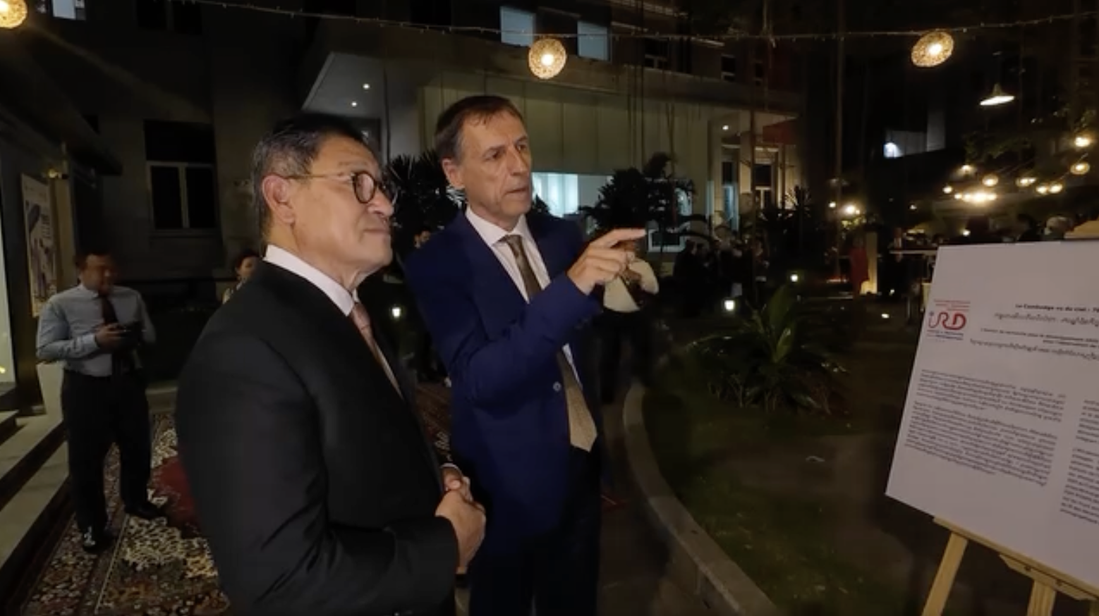
- Khmer Aerial Photographic Archive (FSPI-R KAPA project, 2023-2024): Presentation of the project during the Kick-Off meeting on November 7th 2023
Thanks Jeff Périgois for this video:
- Wat-Health Project “Floods and Health Risks in Cambodia” (FSPI 2021-2022) aimed to determine how and how changes in the river flood regime affect the distribution of pollutants and cause changes in the biodiversity of pathogens and vectors of water-related diseases, ultimately with effects on health, agricultural production and the environment. The project brought together 4 IRD UMRs (G-EAU, Mivegec, Espace-Dev and IGE) as well as partners in Cambodia (the Pasteur Institute of Cambodia, the Institute of Technology of Cambodia and the Royal University of Agriculture). Due to its multidisciplinary nature, this research topic required the coordination of multiple overlapping themes. The film Wat-Health returns to this multidisciplinary adventure through the point of view of its speakers who show some interests and difficulties. Director: Aurélie Surjus Operator: Simon Guyomard © IRD 2023
- 08/2022: Meriem M’Zoughi introduce the OHARAT Project (funded by the FSPI OHSEA)
- 21/10/2021: Vincent Herbreteau (IRD) et Florian Girond (IRD-IPC) présentent le projet SCO ClimHealth à la Trimestrielle du Space Climate Observatory (SCO)
- 10/2021: Animated presentation of our ClimHealth Project (funded by CNES, 2020-2022) (https://www.spaceclimateobservatory.org/climhealth-yangon)
(Discussion organized by Alliance française de Bangkok)
- 12/02/2021: Interview of Vincent Herbreteau, about our contribution to Covid-19 response in Cambodia working on data management and knwoledge transmission through the construction of a COVID dashboard (https://covid.geohealthresearch.org/)
(funded by AFD ECOMORE II – Topup Covid: supporting front-line laboratories in southeast Asia)
- 2019: ECOMORE II Project (funded by AFD): Visit of the schools where entomological surveys are conducted. Field survey is necessary to observe the environment, record landscape description before doing spatial analyses (Images taken by Vincent Herbreteau, IRD)
- 12/2017: Florian Girond présente ses travaux de thèse sur la mise en place d’un système d’information géographique pour la détection précoce et la prédiction des épidémies de paludisme à Madagascar (Travaux réalisés à l’Institut Pasteur de Madagascar, en collaboration avec l’UMR Espace-Dev).
- 16/11/2017: Christophe Révillion (Univ. Réunion, Station SEAS-OI) présente le Projet Sentinel-2 Malaria, et plus spécifiquement la création automatisée d’indicateurs environnementaux à partir des images satellite Sentinel-2 pour la surveillance sanitaire.
(Financé par le CNES TOSCA, 2017-2019)
08/2012: Stéphane Dupuy (Cirad, TETIS) presents our landscape study of the distribution of rodents in South-East Asia at the GEOBIA Conference: “Land-cover dynamics in Southeast Asia: Contribution of object-oriented techniques for change detection“. This work was realized in the frame of the ANR CEROPath Project.
Private: Instagram Demo – Customizer
Whoops! No connected account found. Try connecting an account first.
This is a mif demo page created by plugin automatically. Please don’t delete to make the plugin work properly.
Private: Facebook Demo – Customizer
Warning: Undefined variable $page_access_token in /home/geohealtym/www/wp-content/plugins/easy-facebook-likebox/facebook/frontend/easy-facebook-likebox.php on line 461
No account found, Please enter the account ID available in the dashboard
This is a Facebook demo page created by plugin automatically. Please do not delete to make the plugin work properly.
Applications
Development of Health Information Systems
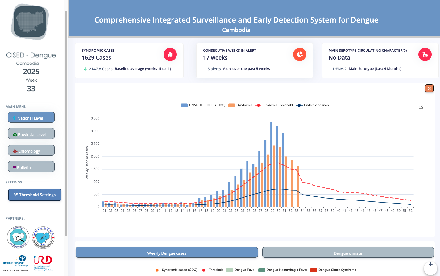
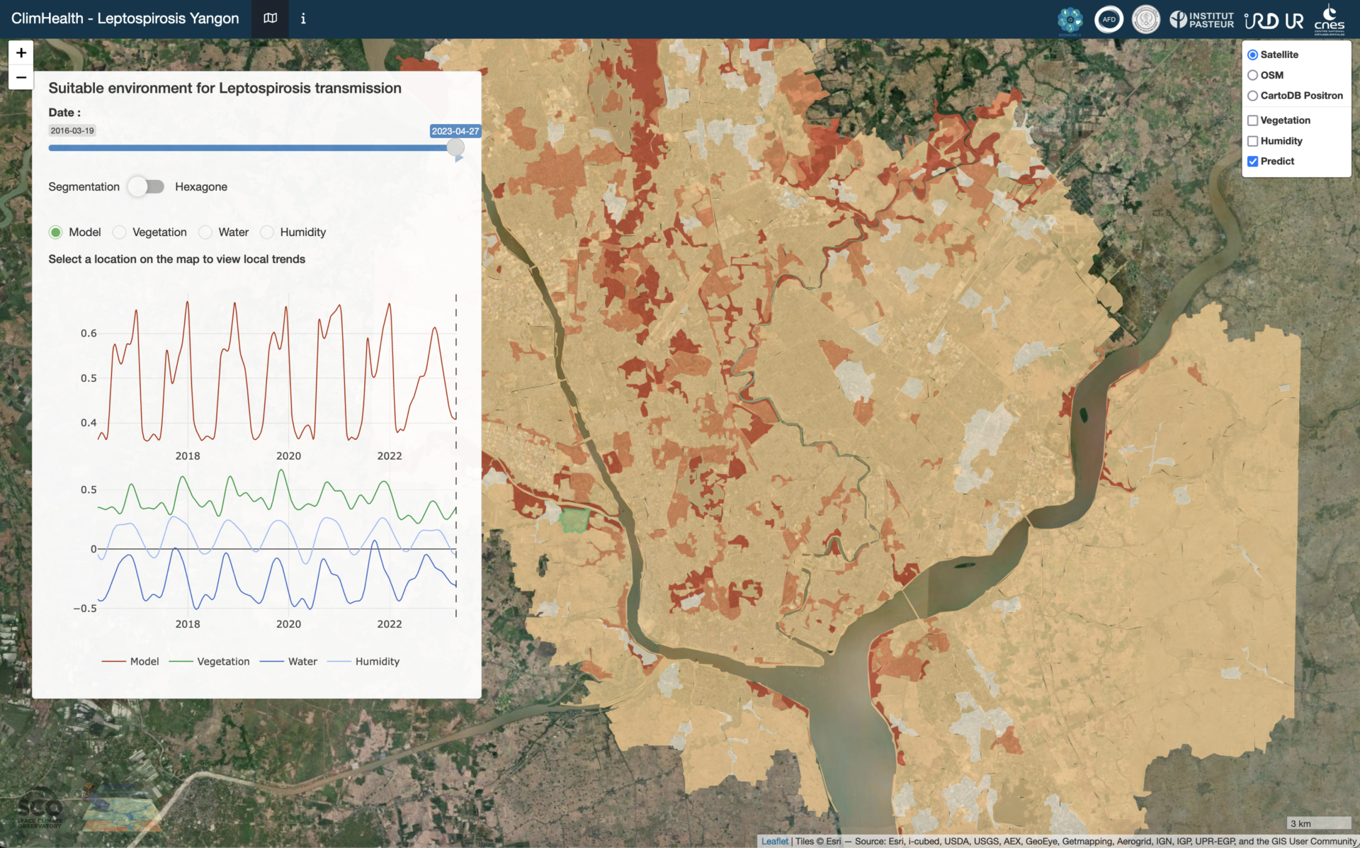
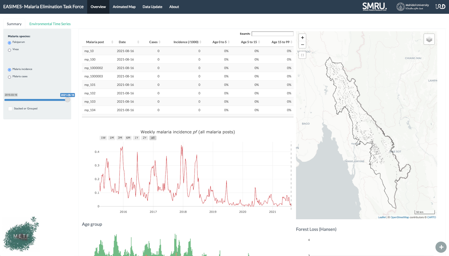
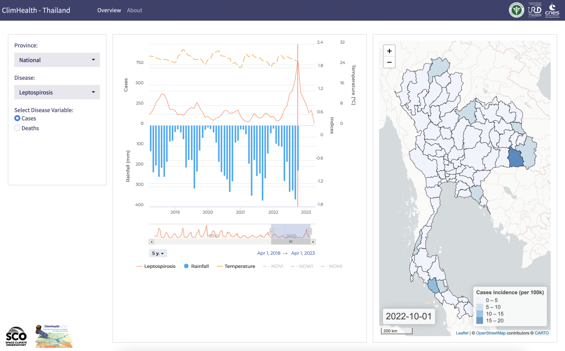
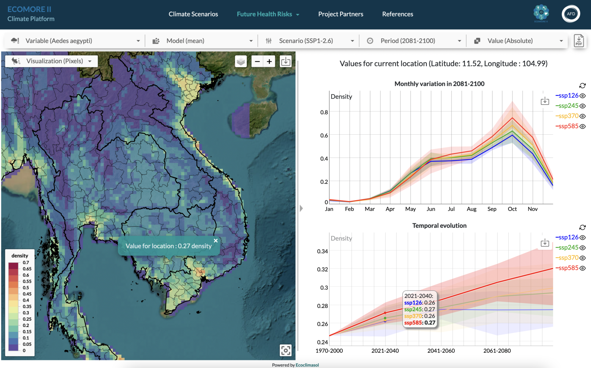
Development of COVID dashboards
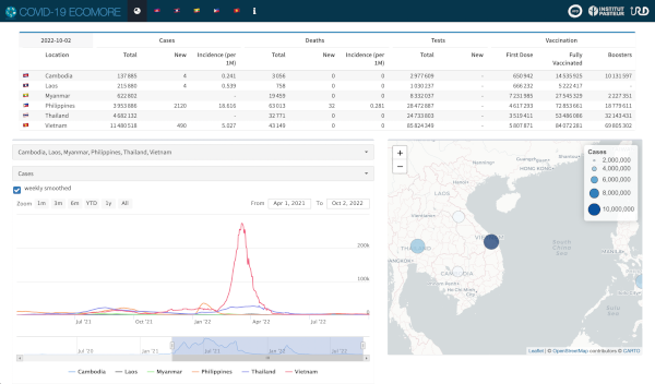
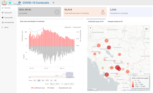
Spatial data tools
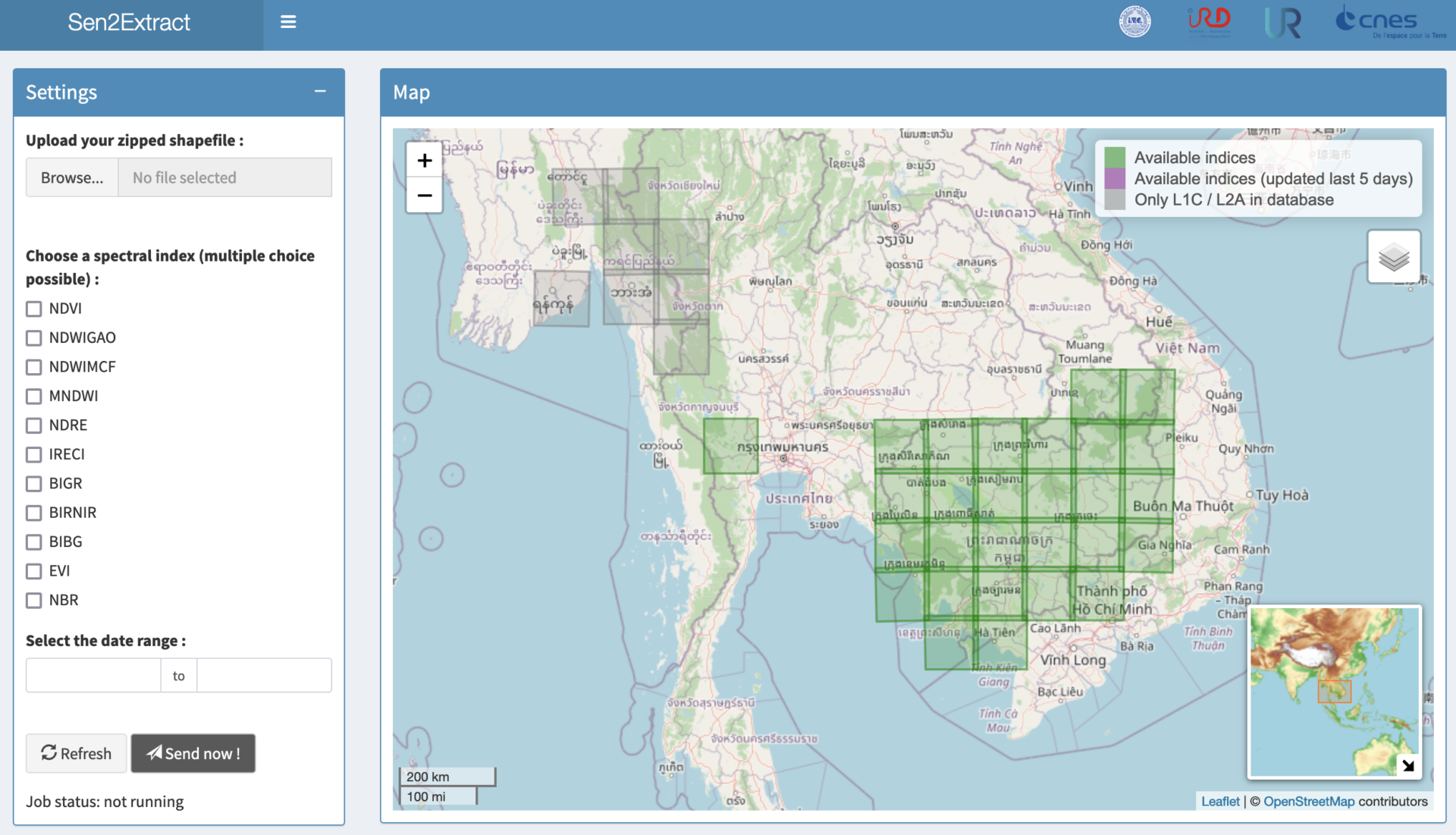
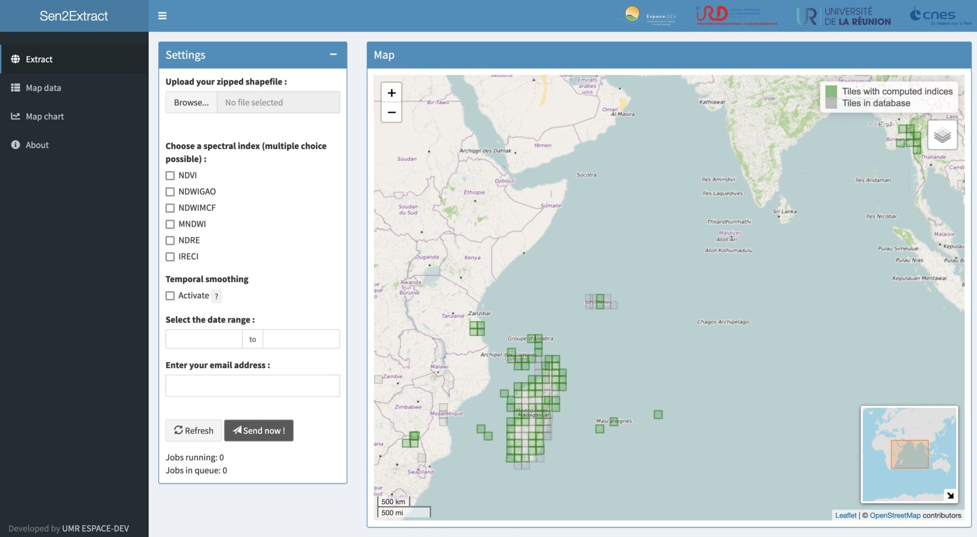
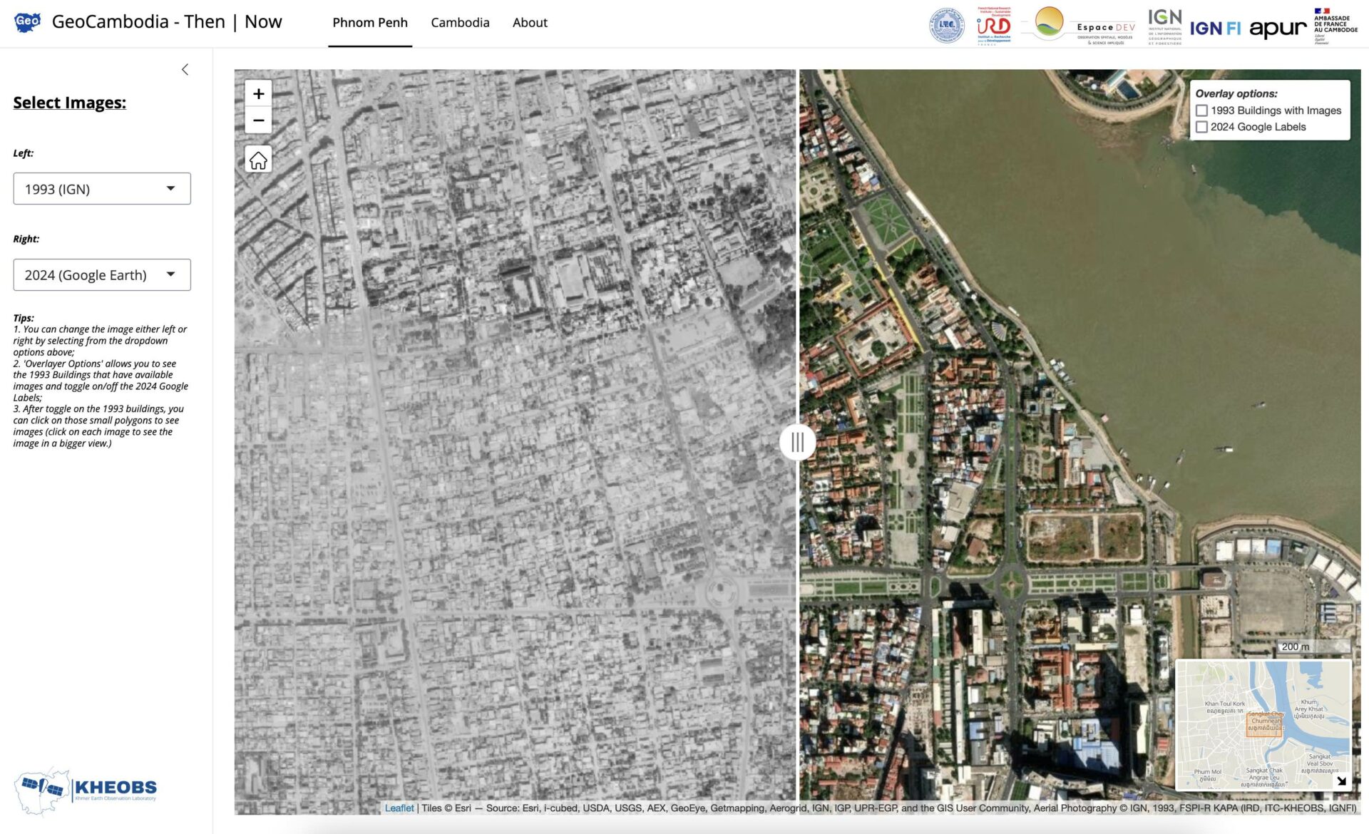
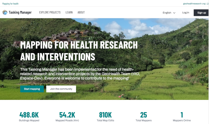
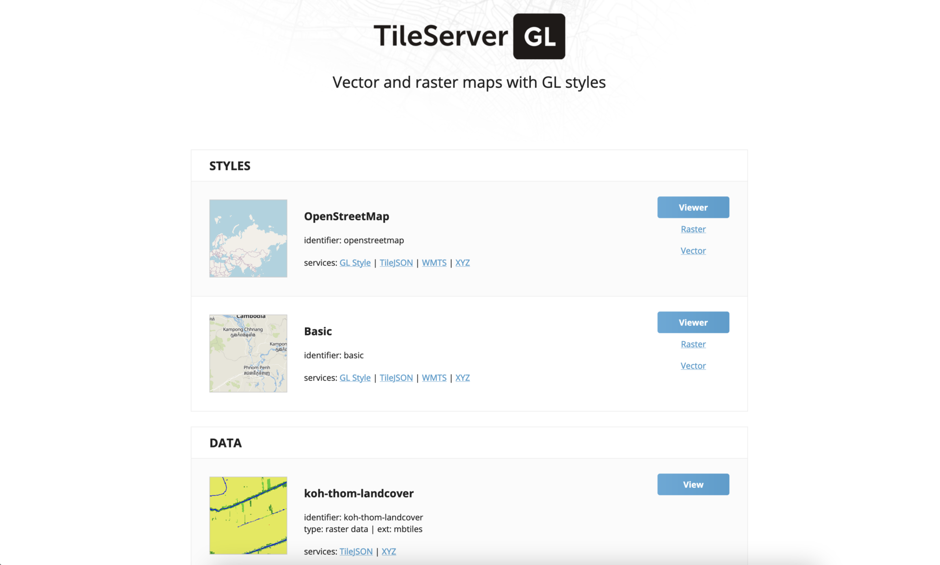
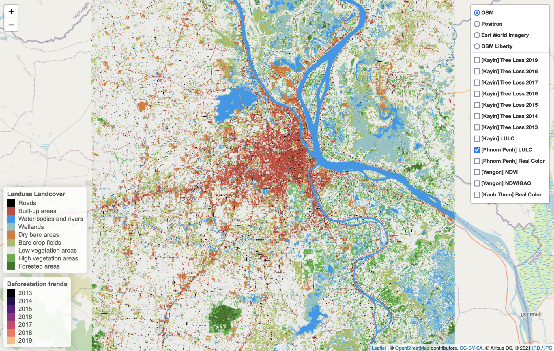
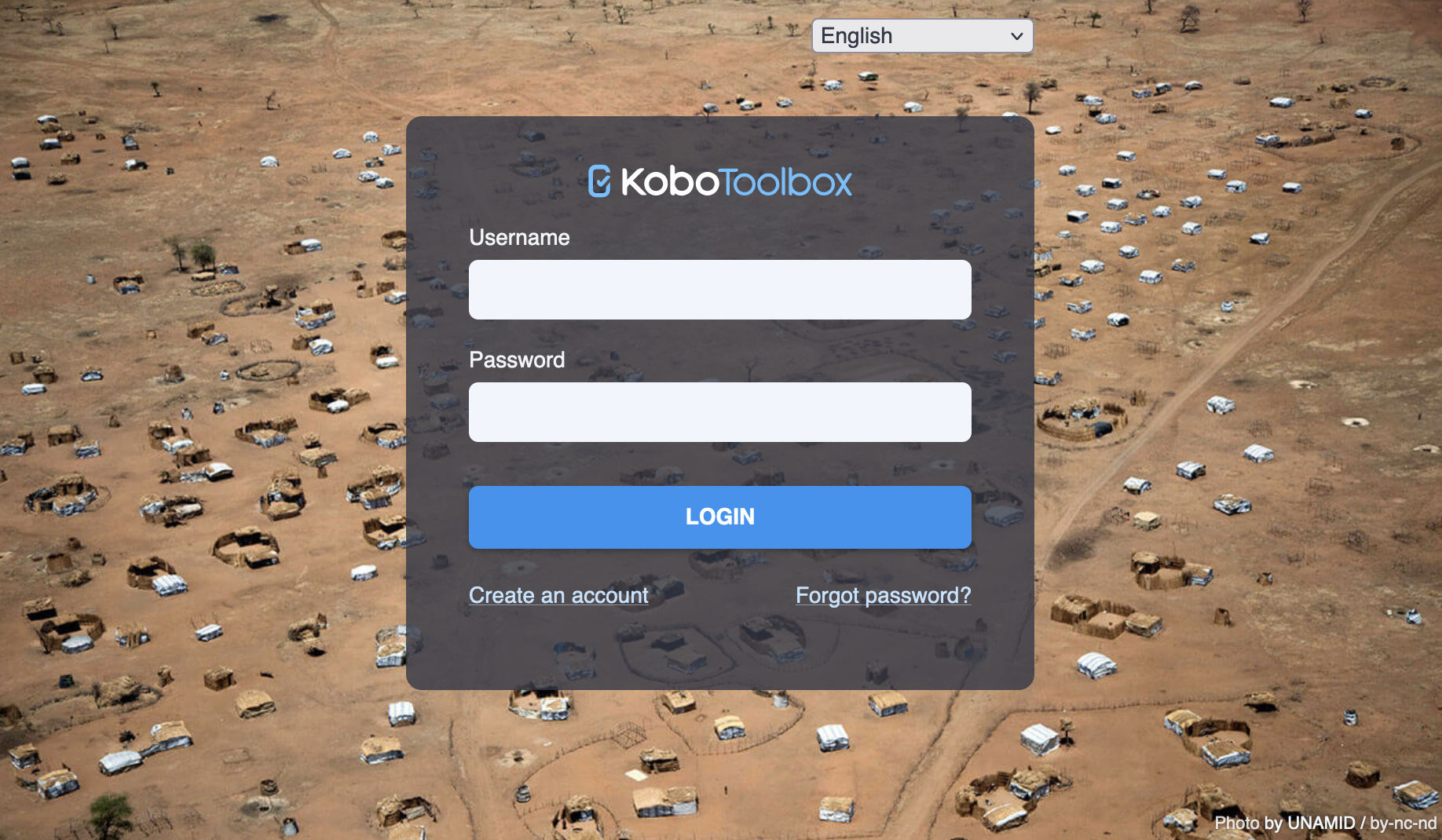
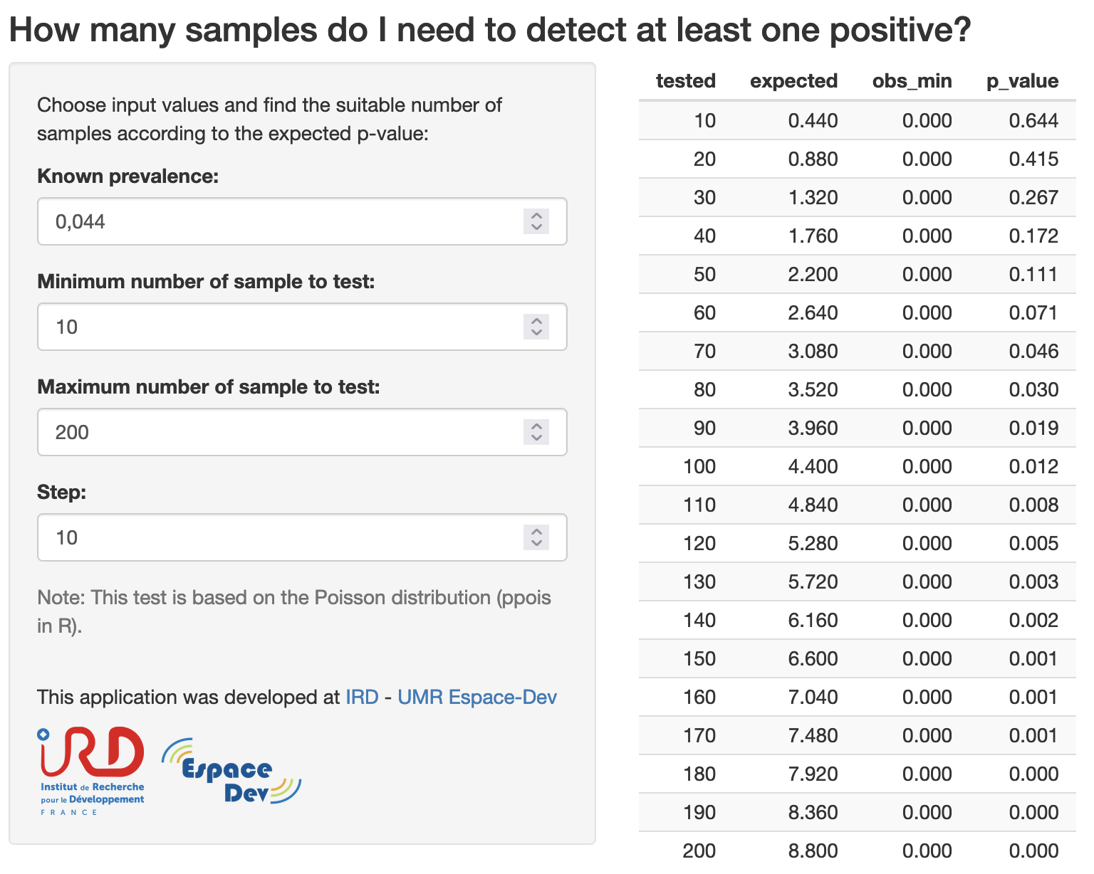
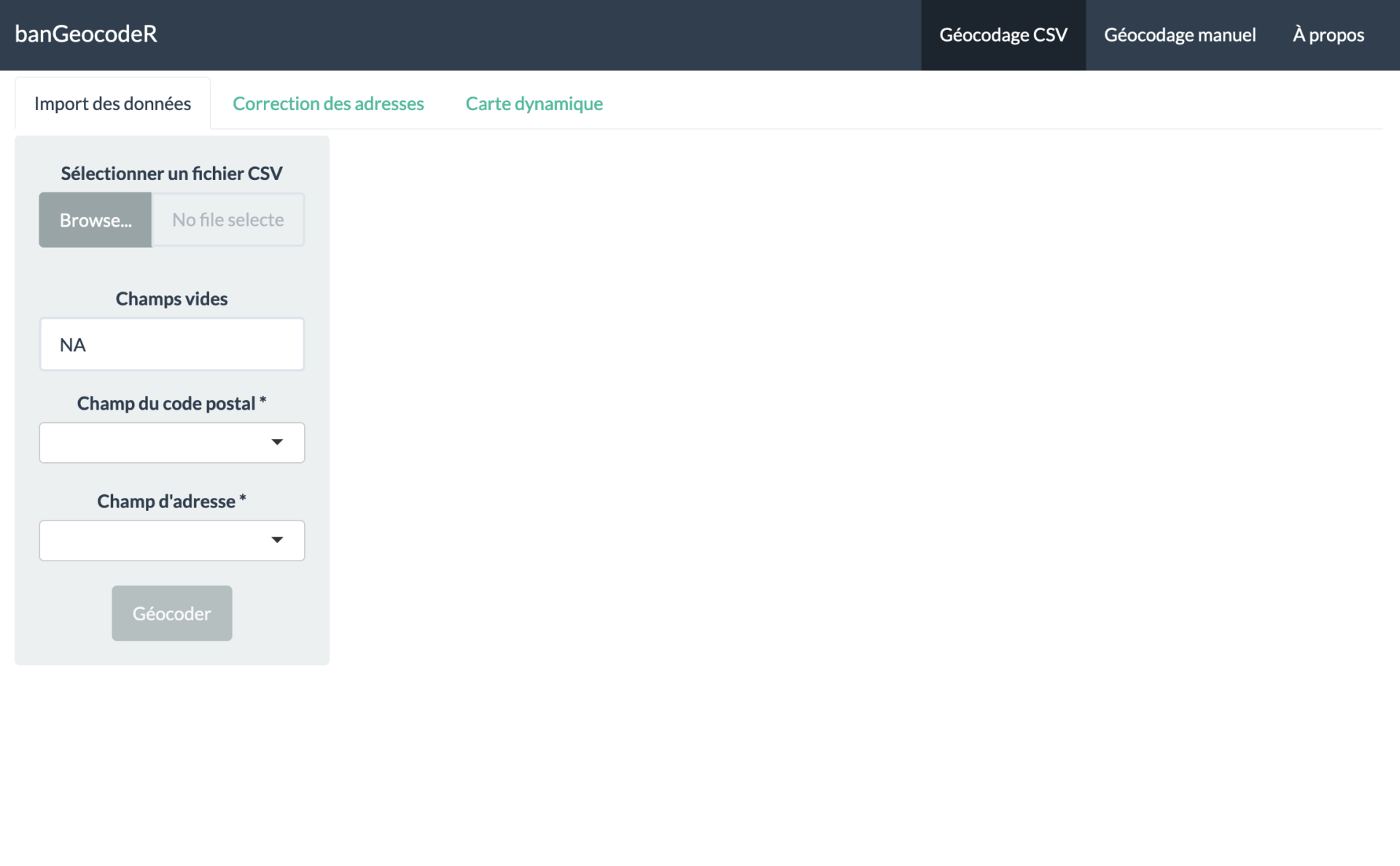
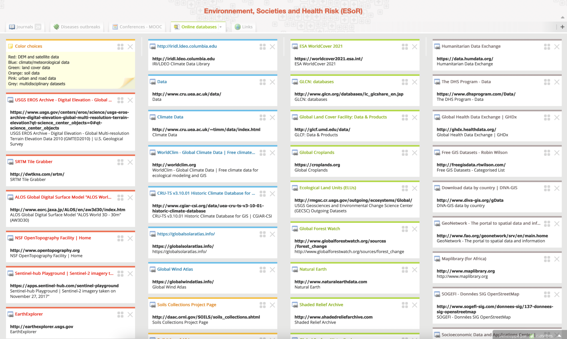
Portfolio Category: Application

#364
QGIS tutorial
based on free data, with Cambodia as an exam

#354
GeoHealth – KHEOBS Team in Cambodia
Vincent Herbreteau
GeoHealth team leader, Health Geographer
Researcher at IRD - UMR Espace-Dev, GeoHealth Team, KHEOBS Laboratory, Phnom Penh, Cambodia


Chendavatey Pok
Project investigator
Medical Doctor (MD), Project investigator at IRD Cambodia, GeoHealth Team, KHEOBS Laboratory at ITC, Phnom Penh, Cambodia
Claire Teillet
Postdoctoral Researcher
Postdoctoral Researcher in Remote Sensing & Vector-Borne Disease Modeling, at IRD Cambodia, GeoHealth Team, KHEOBS Laboratory at ITC, Phnom Penh, Cambodia
Chamroeun Yorngsok
R Developer
Engineer at IRD Cambodia, GeoHealth Team, KHEOBS Laboratory at ITC, Phnom Penh, Cambodia
George Ge
Head of Engineering
Engineer at IRD Cambodia, GeoHealth Team, KHEOBS Laboratory at ITC, Phnom Penh, Cambodia
Sreypich Chy
Geomatician
Geomatician at IRD Cambodia, GeoHealth Team, KHEOBS Laboratory at ITC, Phnom Penh, Cambodia
Ranny Rith
Socio-anthropologist
Associate researcher at IRD Cambodia, GeoHealth Team, KHEOBS Laboratory at ITC, Phnom Penh, Cambodia
Vannak Ann
KHEOBS Co-Director, Hydrologist
Vice-Dean, Lecturer and Researcher at ITC - Water and Environment Research Unit, KHEOBS Laboratory, Phnom Penh, Cambodia

Thibault Catry
KHEOBS Co-Director, Remote sensing expert
Research engineer at IRD – UMR Espace-Dev, KHEOBS Laboratory, Phnom Penh, Cambodia
Associated members
Florian Girond
Project coordinator, Health Geographer
International Technical Expert (ETI) at the Center for Disease Control (CDC) of the Ministry of Health of Cambodia
Christophe Révillion
Remote sensing and GIS expert
Engineer at Université de La Réunion - UMR Espace-Dev, SEAS-OI, Saint-Pierre, La Réunion, France
Former members
Sokeang Hoeun
Geomatician
Former Engineer at IRD Cambodia, GeoHealth Team, KHEOBS Laboratory at ITC, Phnom Penh, Cambodia
Meriem M'zoughi
Socio-anthropologist
Former Researcher at IRD - UMR Espace-Dev, GeoHealth Team, Phnom Penh, Cambodia
Lucas Longour
Geomatician
Freelance geomatician, formerly Engineer at IRD - UMR Espace-Dev, GeoHealth Team, Phnom Penh, Cambodia
#298
Contents
Install QGIS
WordPress Theme
GeoHealth Research on Facebook
[custom-facebook-feed]
Tutorial test
Tutorial for working with
QGIS software
Vincent Herbreteau, IRD, UMR ESPACE-DEV (vincent.herbreteau@ird.fr) Arnaud Vandecasteele, GeoLab.re (arnaud.vdc@geolab.re)
Tutorial QGIS – Composing map layouts
5. Composing map layouts
Map composition (layout) is realized in the Layout Composer.
Exercise: Compose the map layout of neonatal mortality rate in Cambodia (number of deaths during the first 28 completed days of life per 1,000 live births in a given year or period)
-
-
- First you need to render and symbolize your data in the map canvas as you want them to appear in a the map layout
- Create a Print Layout
- Project / New Print Layout…
- Give a name to your layout and click OK
- A right-click on the white page allows to open Page properties and set up the page size (for example A4 landscape)
- Add your map:
- Go to “Add item” Menu / Add Map or Click the button “Add a new map to the layout”
- Draw the extent of map on your canvas
- The map from your QGIS is displayed
- Use the “Move item content” button to move you map within its box
- You can check “Lock layers” and “Lock styles for layers” to fix your map
- You can redo add map to add a second one. Then, you need to go back to GIS main window to choose the display of your map canvas you want to show in the second map
-
-
-
- Add a scale bar:
- Go to “Add item” Menu / Add Scale Bar
- Place your scale bar on the map
- When the scale bar is selected, you can adjust its properties in the Item Properties window
- Choose the style of the scale par in “Main properties”
- Choose the Units: here: 1 km
- Choose the number of Segments: here 50 units
- You can further adjust fonts, margins, etc.
- Add a scale bar:
-
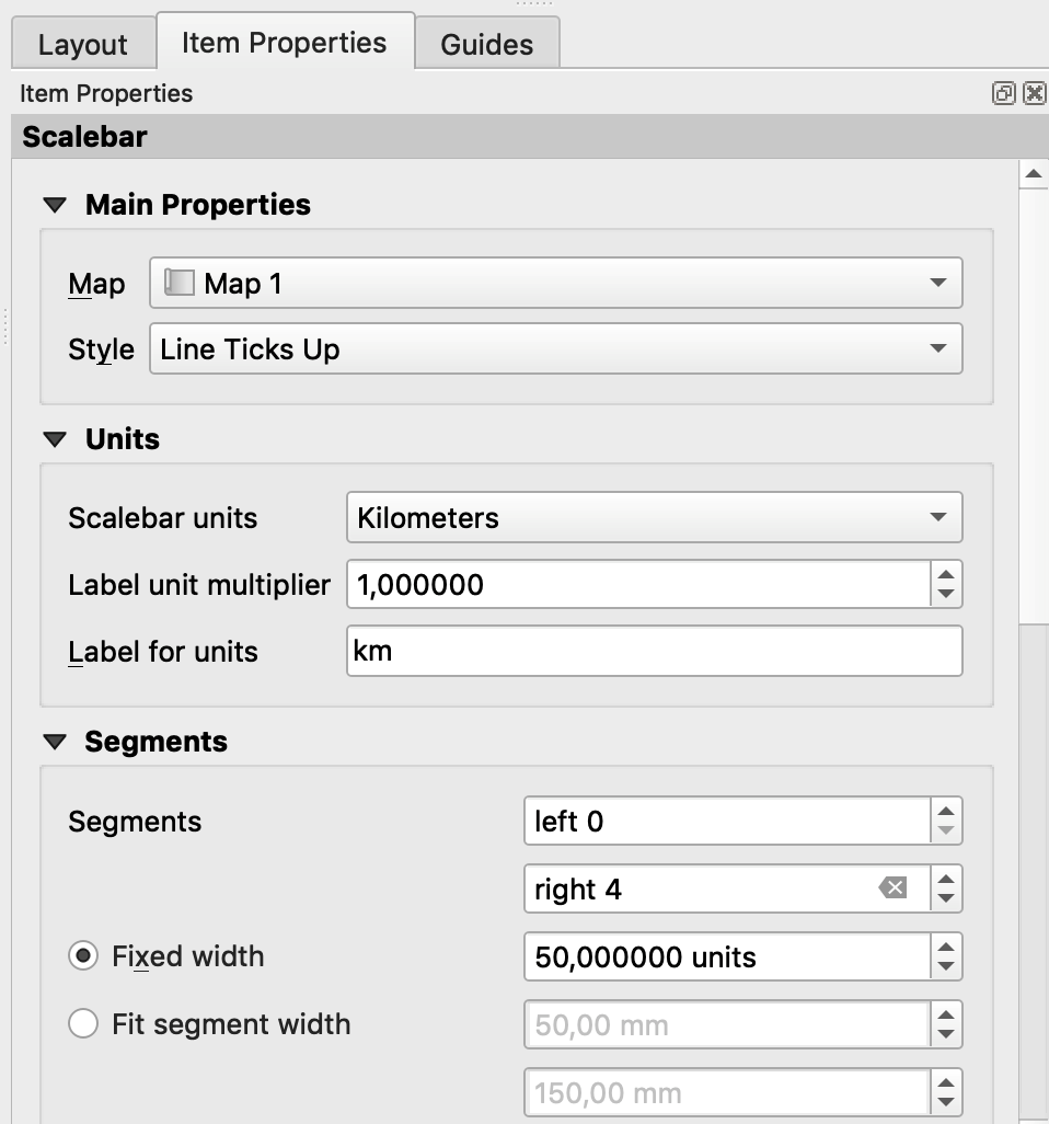
-
-
- Add a legend:
- Go to “Add item” Menu / Add Legend
- Place your legend on the map
- When the legend is selected, you can adjust its properties in the Item Properties window
- In the Legend items: uncheck “Auto update” to remove some parts of the legend or reorder
- You can double-click on a layer name to modify it
- You can further adjust fonts, margins, etc.
- You can uncheck background for a transparent one
- Add a legend:
-
-
-
- Add a North arrow:
- Go to “Add item” Menu / Add Picture
- Place the picture on the map
- In the “Search Directories”, look for a compass or North arrow
- Add a North arrow:
-
-
-
- Add Text for title, sources, etc.
- Go to “Add item” Menu / Add Label
- Add Text for title, sources, etc.
-
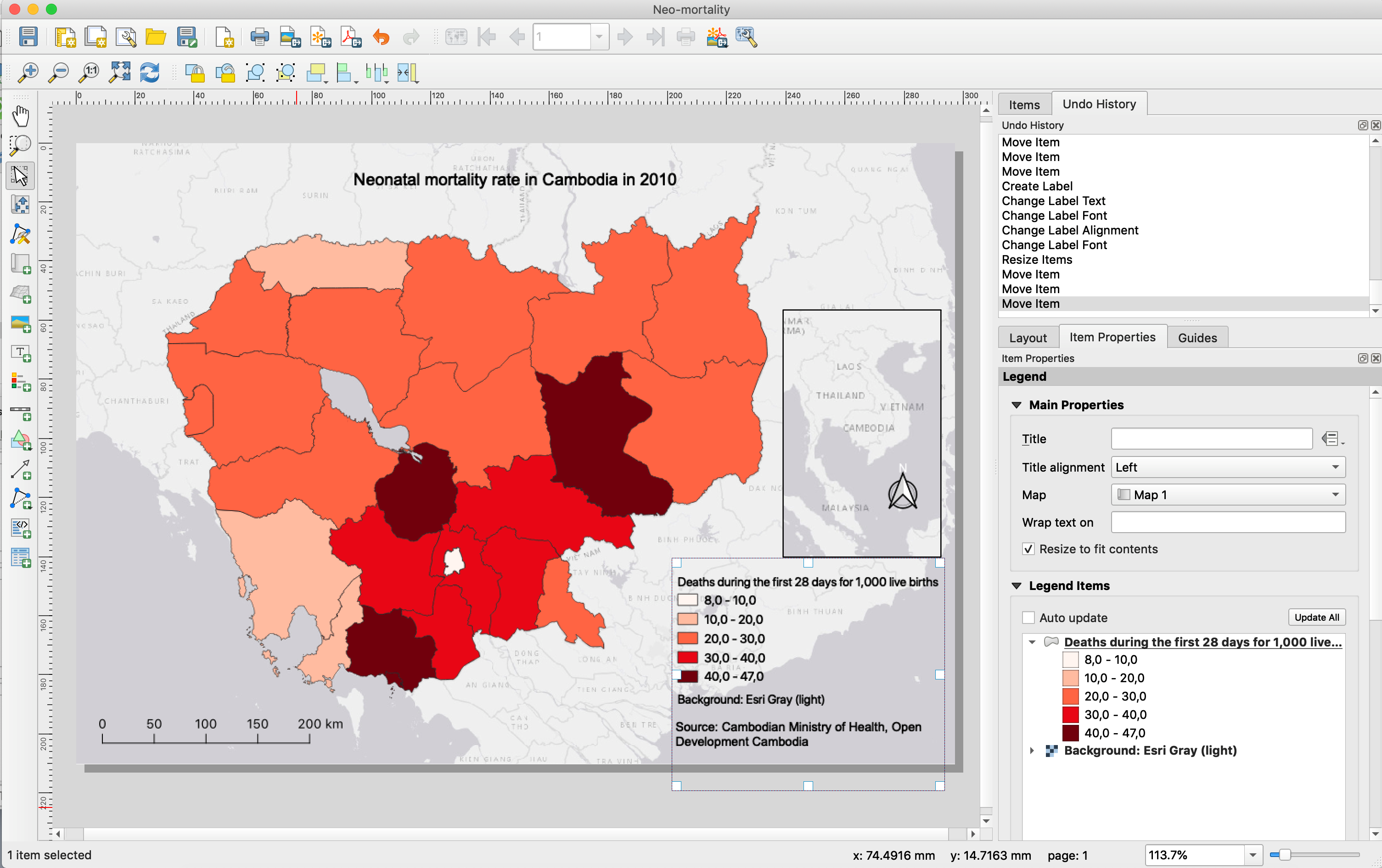
-
-
- Export maps:
- In the Layout tab, should the export resolution (300 dpi is advised for fine printing)
- Export as image or as pdf, depending on your needs
- Export maps:
-
Tutorial QGIS – Using raster data
4. Using Raster Data
In this exercise, we will use a Digital Elevation Model (DEM), called SRTM (Shuttle Radar Topography Mission), provided by NASA and NGA (formerly NIMA).
4.1 Opening and displaying raster data
-
-
- Open the Data Source Manager
 , choose the “Raster” tab and browse to srtm_cambodia.tif
 - Double-click on the name to open the Layer Properties, and go to the Symbology tab
- In Render type, choose “Hillshade” and Apply to view the Elevation data with shadow
- Try also the “Singleband pseudocolor” for a color view. You can adjust the classification mode and increase the number of classes. You can choose the color ramp and invert colors.
- Open the Data Source Manager
-
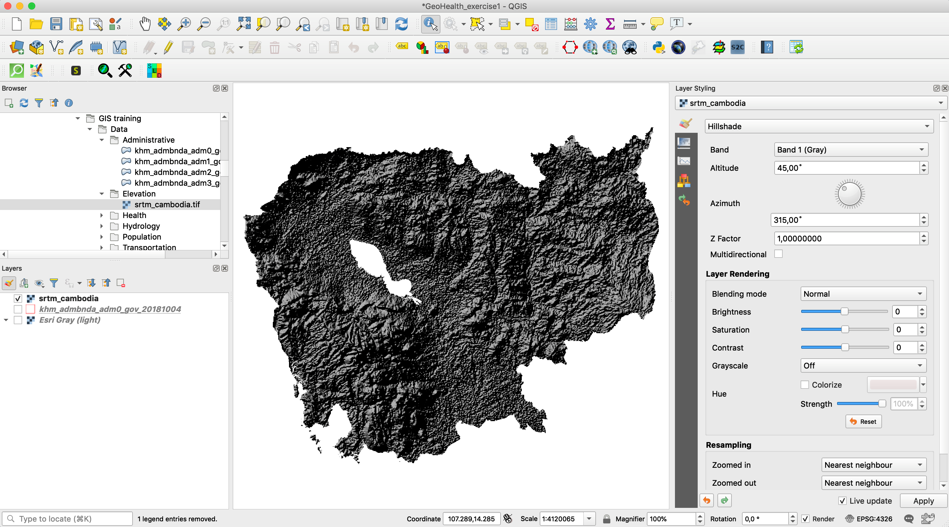
4.2 Clipping a raster data
QGIS offers the possibility to cut a raster according to the contour of vector layers.
Exercise: Extract the SRTM on Mondolkiri province (east of Cambodia)
-
-
- Create a shapefile layer of Mondolkiri
- Open the province layer: khm_admbnda_adm1_gov_20181004
- Select Mondolkiri province
- Right-click on the name of the layer / Export / Save Selected Features As…
- Browse to your folder and save the Mondolkiri.shp layer
- Raster / Extraction / Clip Raster by Mask Layer…
- Input layer = srtm_cambodia.tif
- Mask layer = Mondolkiri.shp
- Run
- Create a shapefile layer of Mondolkiri
-
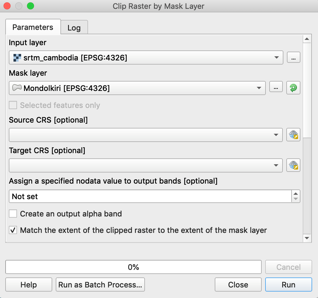
4.3 Changing the projection of a raster
The DEM srtm_cambodia.tif is in WGS84 with units in decimal degrees. To make some calculations related to distances, we will need the meter as a unit. It is therefore necessary to reproject our raster.
Exercise: Reproject the Mondlkiri DEM in the local projected CRS
-
-
- Go to Raster Menu / Projections / Warp (Reproject)
- Input layer = srtm_Mondkiri.tif
- Target CRS: choose the local projected CRS
- Browse to your folder and give a name to the Reprojected raster
-
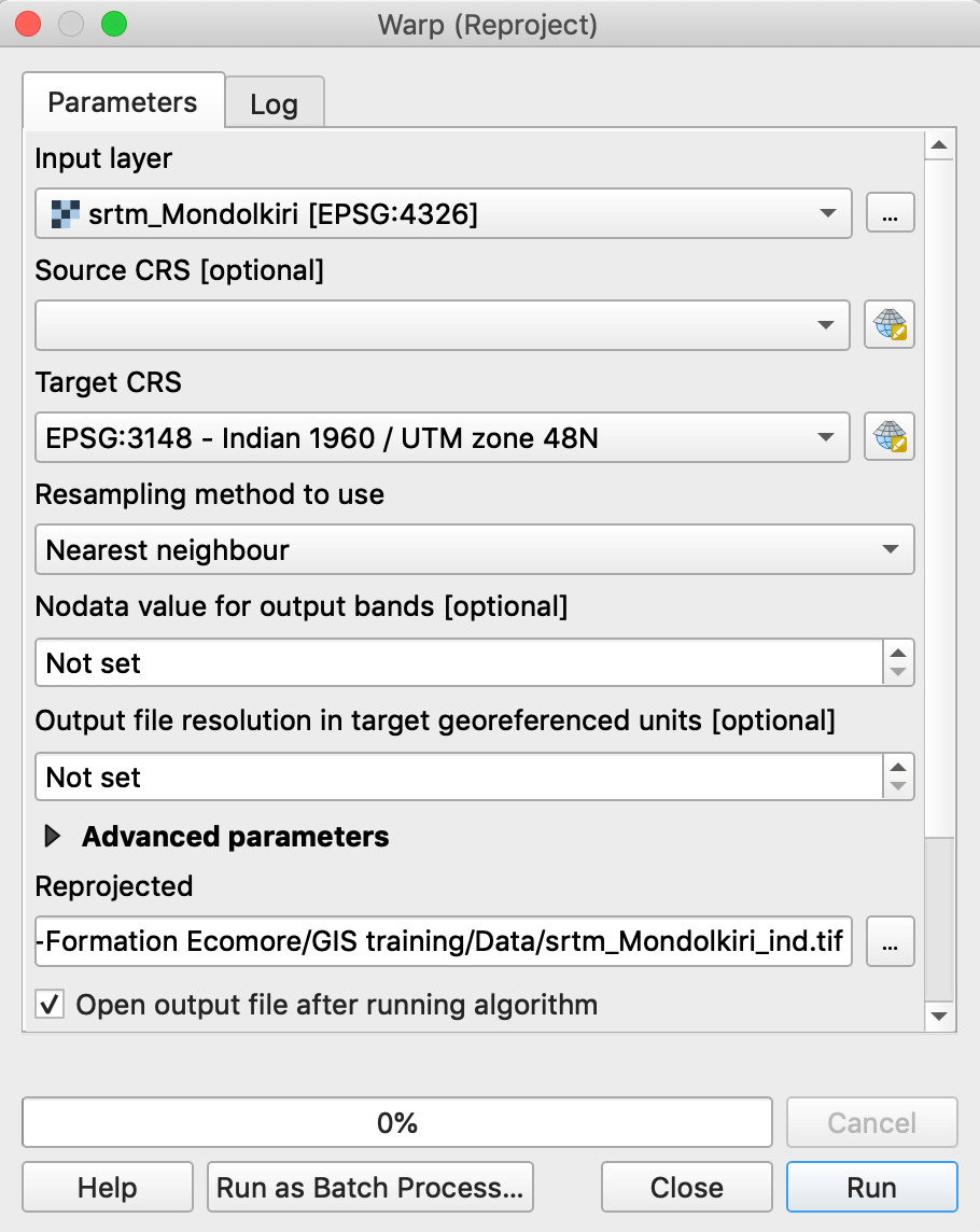
4.4 Deriving information from DEM: slopes, aspect, hillshading, contours
Several tools are provided in the Analysis Menu from the Raster Menu
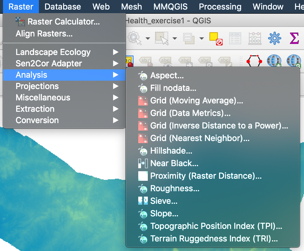
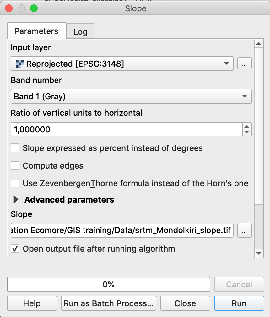
Exercise: Calculate slope and aspect in Mondolkiri province
-
-
- Go to Raster Menu / Analysis / Slope…
- Choose the Mondolkiri DEM
- Browse to your folder and give a name to the raster of slopes
- Run
- The same applies to the calculation of exposure (aspect) and hillshading.
-
Note: Calculating the slope in QGIS is simple. The output is also a raster of the same resolution (90 meters) as the source raster.
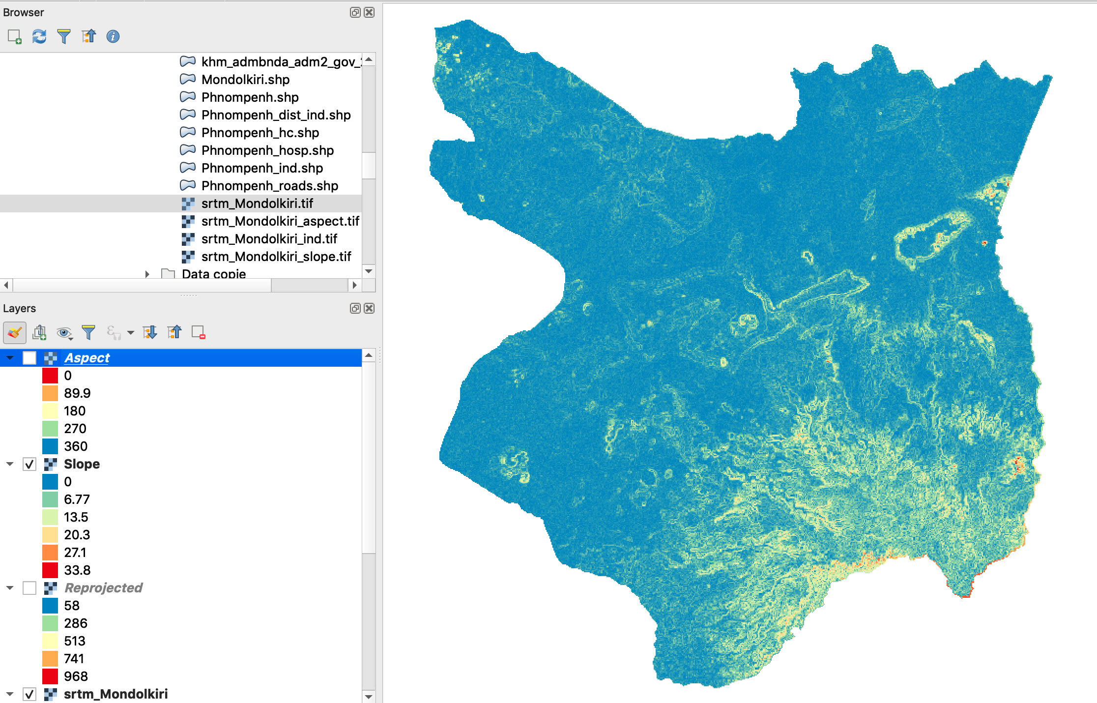
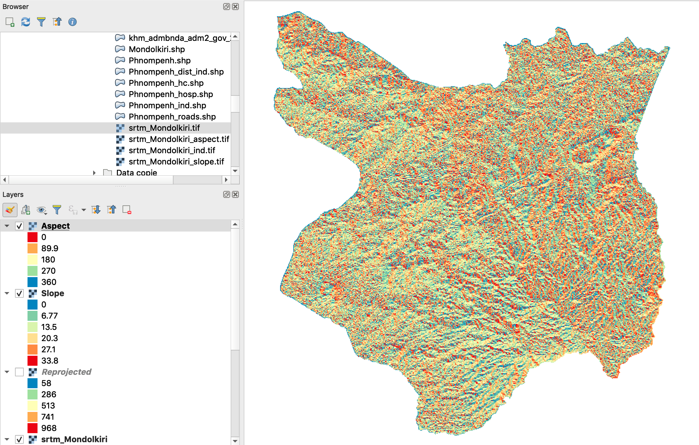
Exercise: Calculate the contour lines of Mondolkiri province
-
-
- Go to Raster Menu / Extraction / Contour…
- Choose the Mondolkiri DEM
- Choose the interval between lines = 100 meters
- Browse to your folder and give a name to the shapefile of contour lines
- Run
-
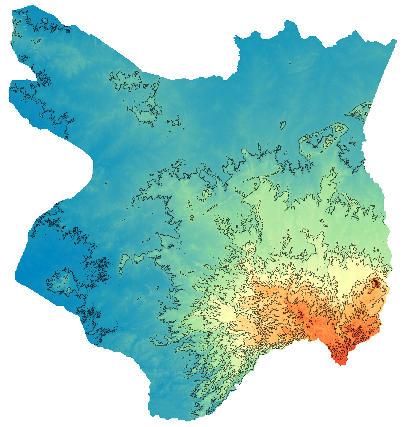
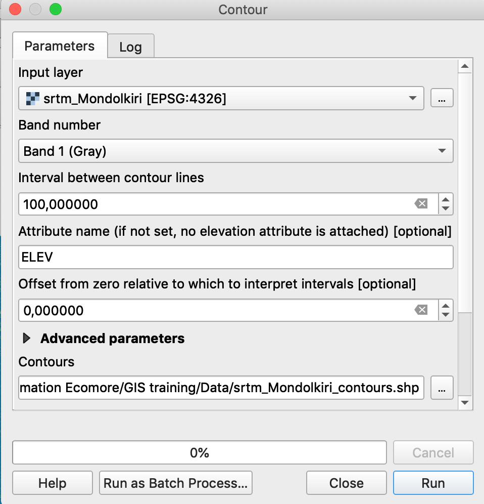
4.5 Raster calculator
The raster calculator allows you to make calculations between several rasters or on the values of a single raster.
Exercise: extract the DEM over 500 meters high
-
-
- Open the raster calculator: Raster / Raster calculator…
- Select the Mondolkiri raster
- Browse to your folder and give a name for the output layer
- Raster Calculator Expression: Double-click the raster name in the “Raster Bands” list to enter its name in the expression then write “> 500”
- OK
-
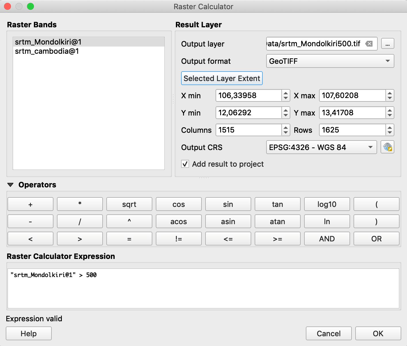
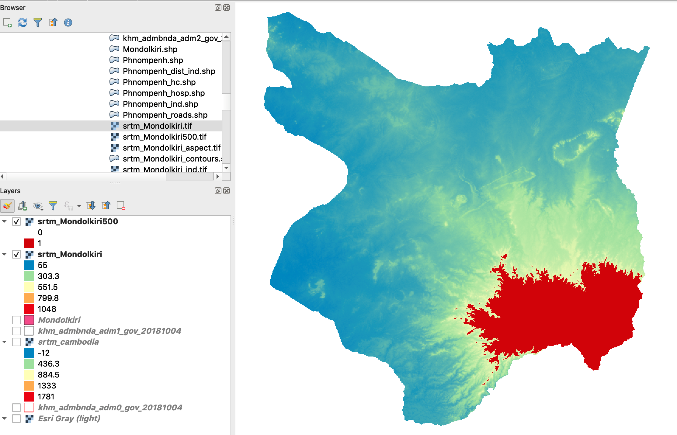
4.6 Downloading and using Sentinel-2 images
Browse and download Sentinel-2 images
We will use here the EO Browser provided by Sentinel Hub and developed by Sinergise:
https://apps.sentinel-hub.com/eo-browser/
Exercise: download and display a Sentinel-2 image from Phnom Penh
-
-
- Open the EO Browser and search for Phnom Penh in the top right search box. Zoom the map to Phnom Penh
- Choose Sentinel-2 L1C as Data source, reduce the maximum cloud coverage to 20%
- Choose a time range and search
-
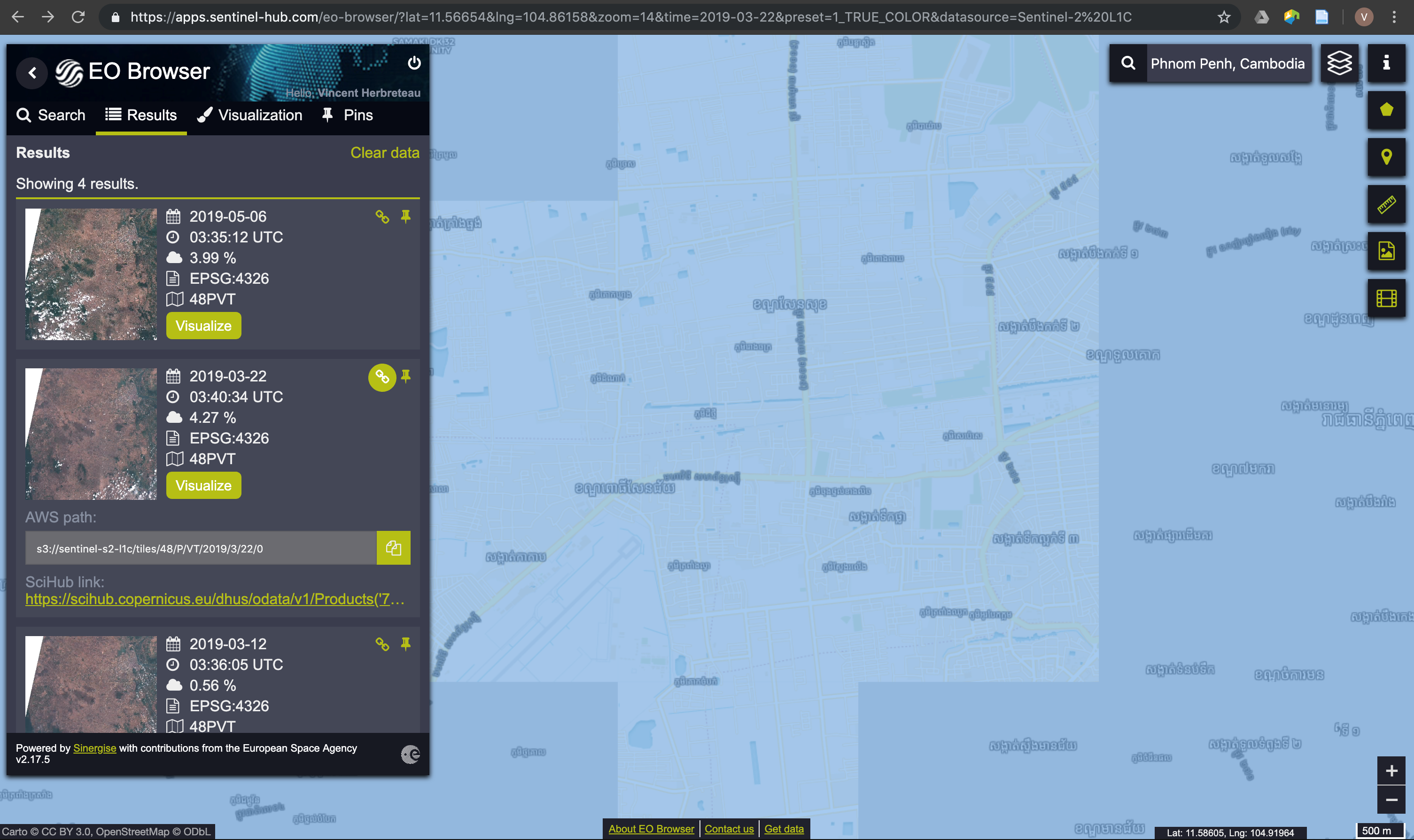
-
-
- Choose one tile among the results and click on Visualize
- Look at the different indices available to observe their distribution
-
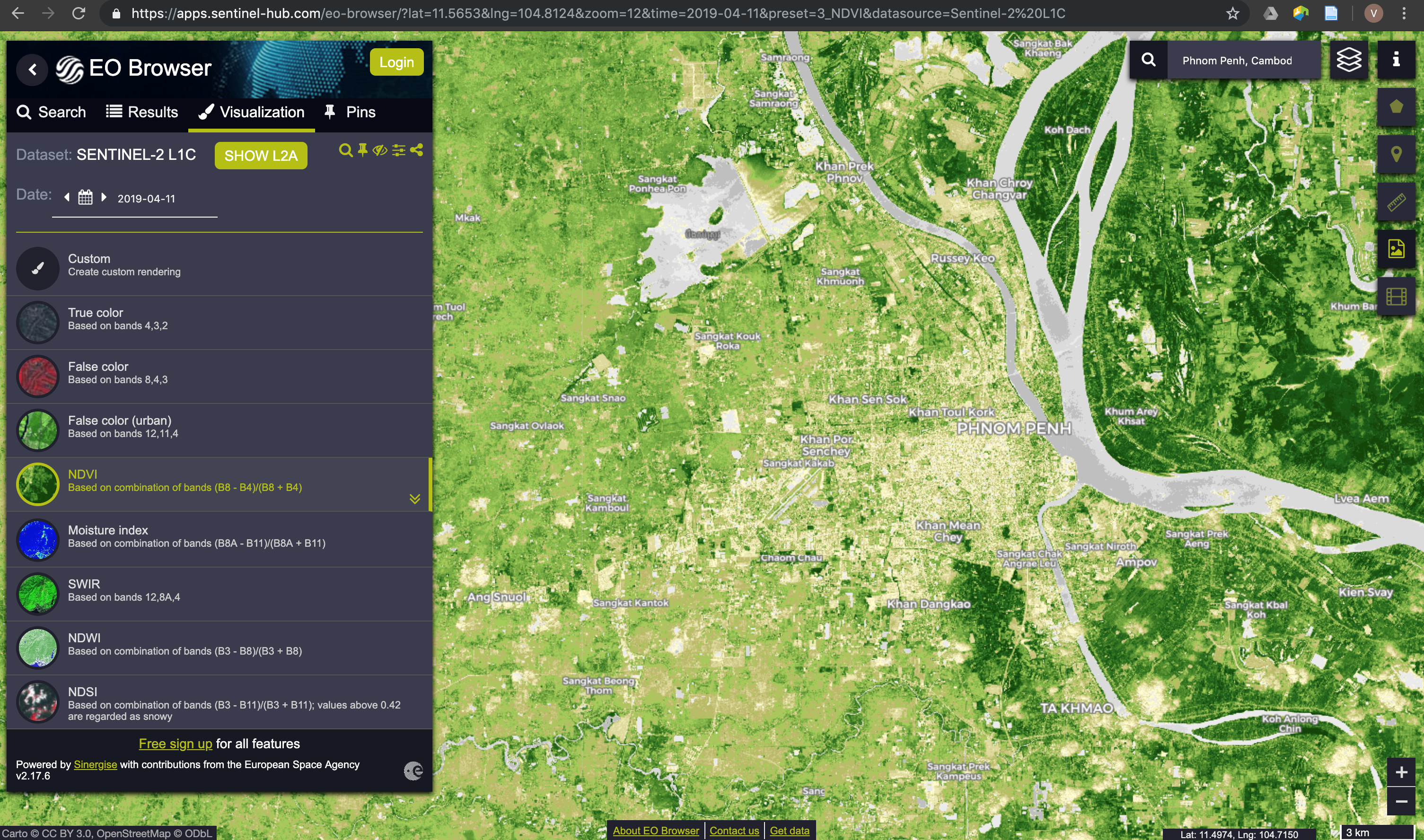
-
-
-
- Click on the download icon
 to get the weblink to download the chosen image
 - Download requires to be registered in the Copernicus Open Access Hub (https://scihub.copernicus.eu/)
- Click on the download icon
-
-
Display a Sentinel-2 image in True color
-
-
- Add the raster bands of your Sentinel-2 images: Menu Layer / Add Layer / Add Raster Layer…
- Browse and choose the different bands to open B02 (Blue), B03 (Green) and B04 (Red)
- Miscellaneous / Build Virtual Raster…
- Choose the 3 input layers
- Run
- Open the layer properties of your virtual raster and go to Symbology tab
- Choose the correct bands for each color and click OK
-
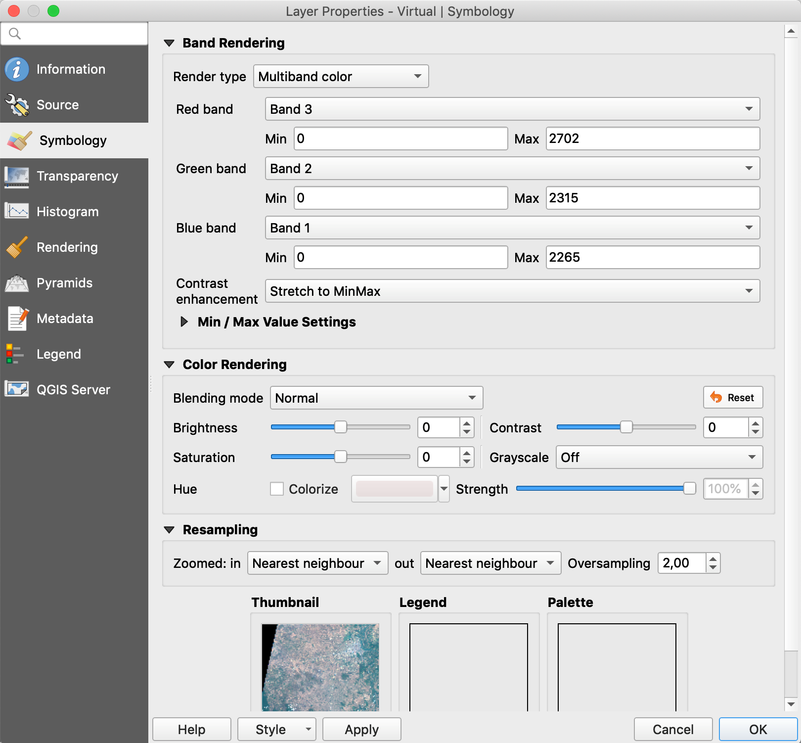
Exercise: Calculate the NDVI of this Sentinel-2 image from Phnom Penh
The normalized difference vegetation index (NDVI) is a simple index that can be calculated from optical satellite images to show the vigor of vegetation.
NDVI = (Near Infrared Band – Red Infrared Band) / (Near Infrared Band + Red Infrared Band)
-
-
- Go to Raster / Raster Calculator
- Browse to your folder and give a name for the NDVI
- Write the equation of NDVI
- OK
- Open the layer properties of your NDVI and go to Symbology tab
- Select Render type = Singleband pseudocolor
- Choose a Red to Green color ramp and a method of classification
- OK
-

Tutorial QGIS – Using vector data
3. Using Vector Data
3.1 Downloading OpenStreetMap data
OpenStreetMap (OSM: www.openstreetmap.org) is an open-access geographic database of the World. You are free to use it for any purpose as long as you credit OpenStreetMap and its contributors.
The QuickOSM plugin, developed by Etienne Trimaille at 3Liz, is the easiest way to access OSM data, through the Overpass API. Users can directly request OSM features over a given extent, by defining the keys, values and boundaries in the Quick Query tab. Users can choose to act directly on the script to best configure their request after clicking on the “Show query” button.
-
-
- Install QuickOSM from the plugins manager
-
Exercise: Download the hospitals of Cambodia
-
-
- Go to Vector / QuickOSM / QuickOSM
- In the Quick query, choose:
- Key = amenity
- Value = hospital
- In = Cambodia
- Run query
- Data will be downloaded as polygon and points shapefiles
- In the “Advanced” list, you can choose the type of data to download (Node / Way / Relation / etc.) or increase the timeout if necessary
- Export the downloaded data as shapefile for further uses
-
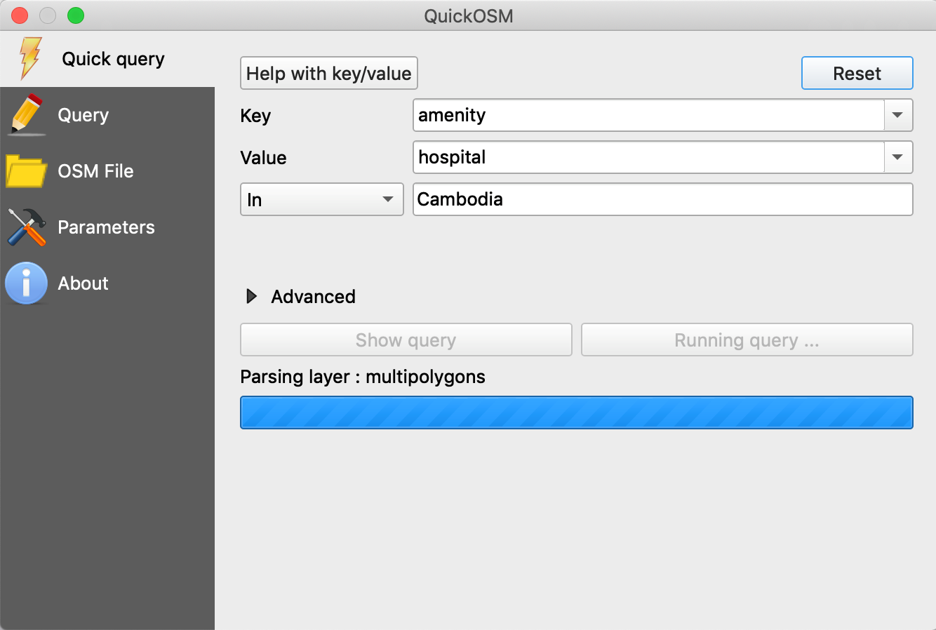
Note: Clicking on the “Help with key/value” will directly open the Map Features page of the OSM wiki: https://wiki.openstreetmap.org/wiki/Mapfeatures
For administrative boundaries, check here the administrative levels by country: https://wiki.openstreetmap.org/wiki/Tag:boundary%3Dadministrative#10_admin_level_values_for_specific_countries
3.2 Joining a data table to a map
In this exercise, we will join the population data (khm_pop_2016_adm3_v2.csv) to the layer of communes khm_admbnda_adm3_gov_20181004.shp based on a common field.
-
-
- Add the layershp to the map
- Add the tablecsv the project. It cannot be directly added by double-click because settings should be carefully checked to ensure a good data format:
-
-
-
-
- Open the Data Source Manager , choose the “Delimited Text” tab and browse to your csv file
- Precise the file format (here, we use custom delimiters and check “Comma”). Also this file has no geometry (Check “No geometry”). Press “Add”.
-
-
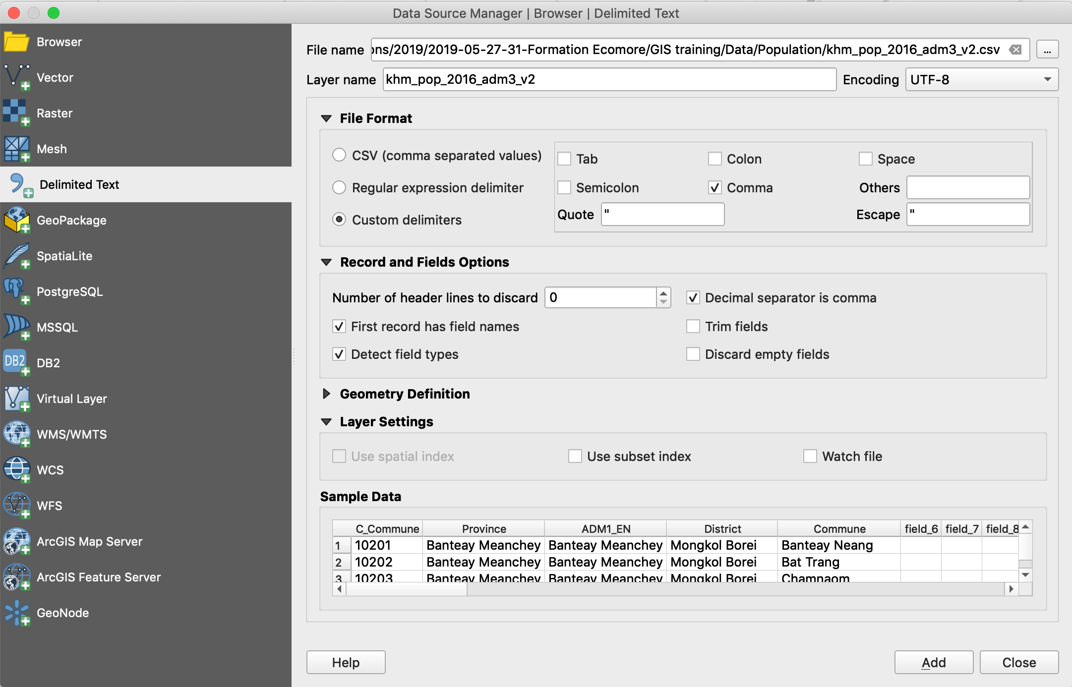
When opening this file with the Open Attribute Table button ![]() (or by right-clicking on its name), you can verify that the data attributes (M, F, T) are in a numeric format (right alignment).
(or by right-clicking on its name), you can verify that the data attributes (M, F, T) are in a numeric format (right alignment).
You can also verify the type of each attribute by opening the Layer Properties window (double-click on the name of the table) and opening the Source Fields tab.
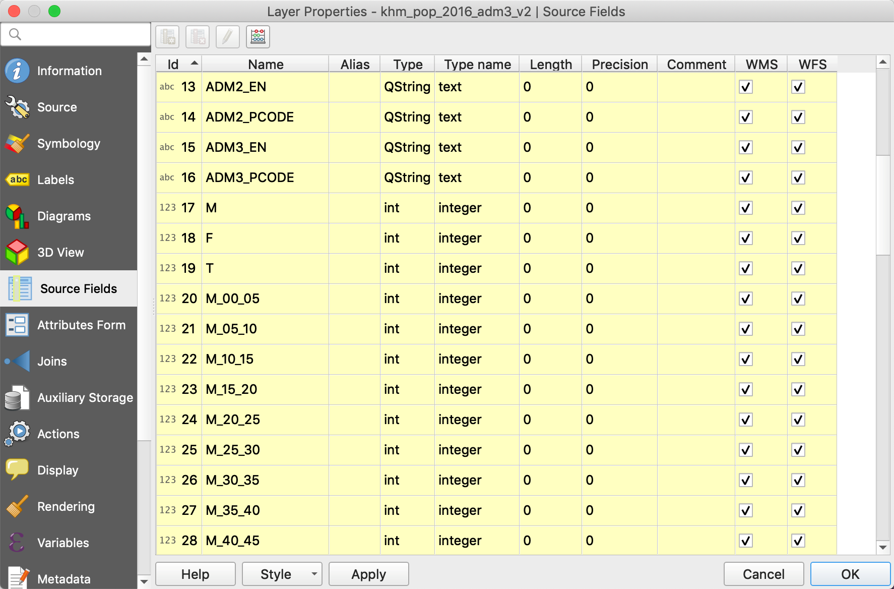
-
-
- Open the Layer Properties window (double-click on the name of the table) of the shapefile in which you want to join the table
- Open the Joins tab and click on the “Add New Join” button (green + button) to add the table
- Select:
- Join layer = khm_pop_2016_adm3_v2.csv
- Join field = ADM3_PCODE
- Target field = ADM3_PCODE
- Check the “Custom Field Name Prefix” and choose a short prefix such as “pop”, otherwise the name of the joined attributes will be too long
- OK
-
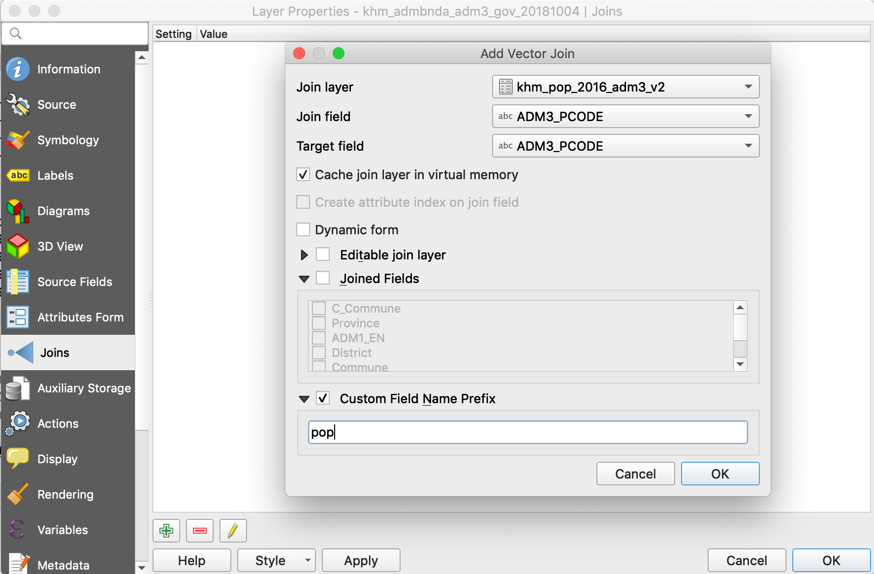
-
-
- Check that the join has enriched the attribute table of the communes layer.
- Save this new layer under a new name to permanently record the information in the attribute table
- Choose a symbology to display population data:
- Open the Layer Styling panel
- Choose “Graduated” for a continuous variable, and select the column to display
- Choose a “Color ramp”, a “Mode” (Equal Interval, Quantile, Natural Breaks, Standard Deviation, Pretty breaks) and click on “Classify”, then “Apply”
-
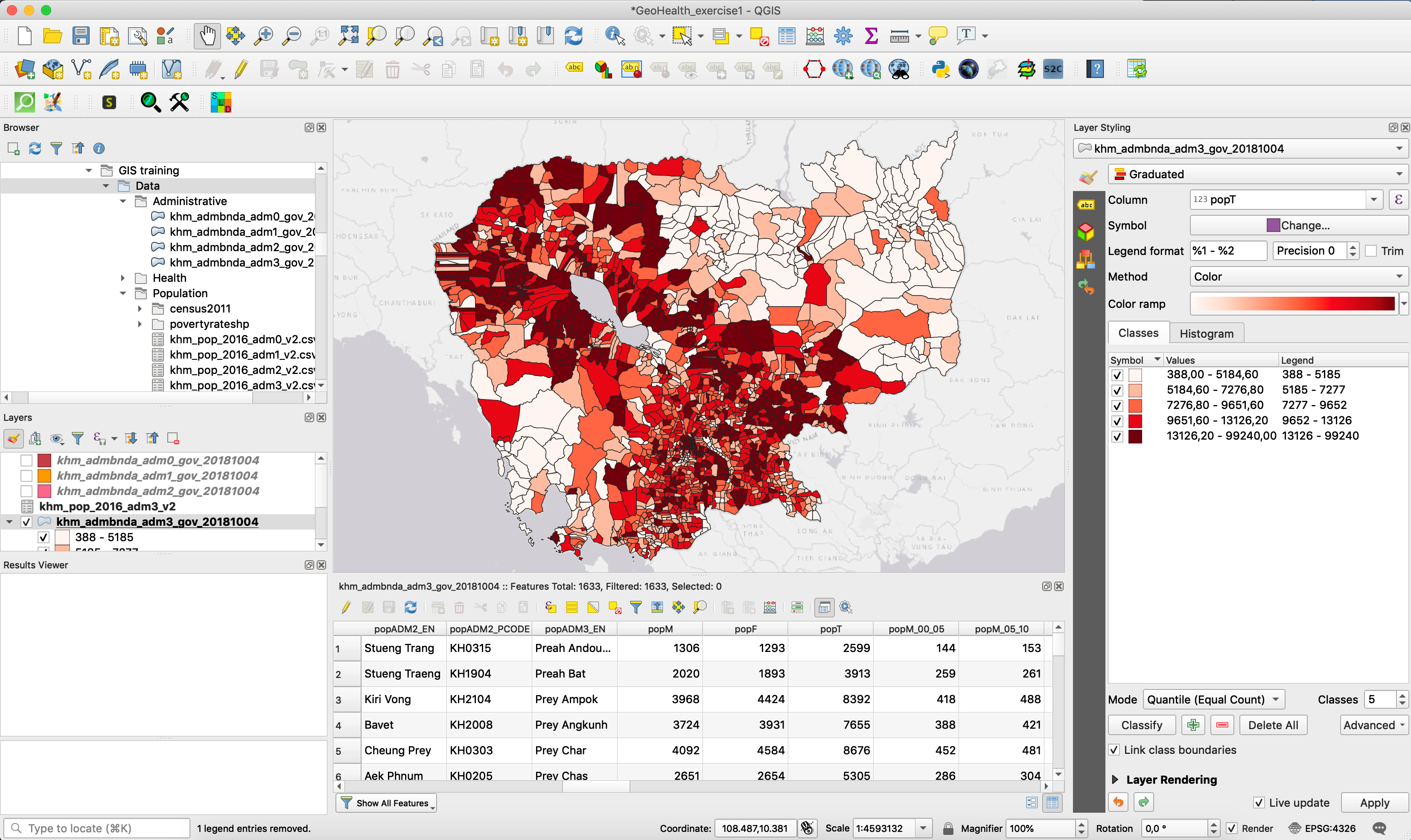
3.3 Creating new attributes in the attribute table
In this exercise, we will calculate the population densities from the Commune layer, which has been enriched with the population data per commune. It will first be necessary to the surface areas of each municipality and then divide the population by the surface area:
-
-
- Open the Attribute Table
 of the Commune layer
 - We will use the buttons above the table dedicated to editing the table:
- Open the Attribute Table
-

-
-
- First click on the pencil to activate the edit mode, the other buttons then become accessible.
- Click on the Open Field Calculator button

-
-
-
- Choose create a new field for Population density as Decimal number
- Choose from the Fields and values list the attribute for Total population "popT"
- Choose the function: here in the Geometry list, double click on $area
- Write the expression: "popT" / $area * 1000000 (multiply by 1 million to have the densities in sq. km)
- The output preview shows that the calculation is indeed consistent
- Click OK
- Finally click on the Pencil button to exit the editing mode and Save.
-
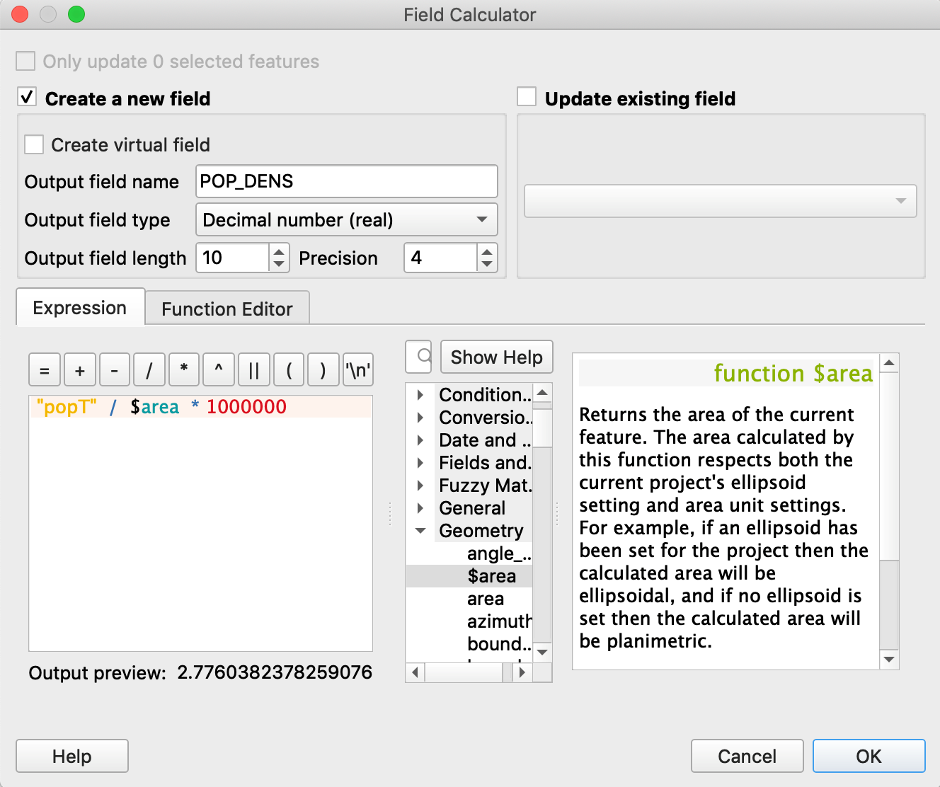
-
- Note: When you switch to edit mode of the attribute table, it is also the shapefile that can be modified.
- Check consistency in the population field of the attribute table or by displaying on the map.
- Note: When you switch to edit mode of the attribute table, it is also the shapefile that can be modified.
3.4 Creating a map from a selection of entities
Exercise: Create a map of Phnom Penh Municipality (province)
-
-
- Open the province shapefile: khm_admbnda_adm1_gov_20181004.shp
- Select Phnom Penh
- Right click on the layer name and choose Export / Save Selected Features As…
- Choose the ESRI format, the destination of your new shapefile, name it
- OK
-
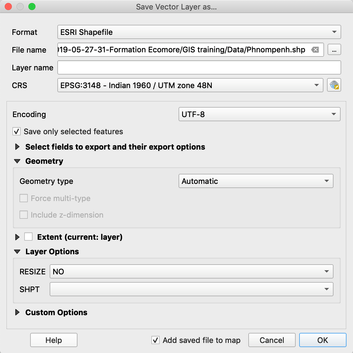
3.5 Intersecting vector layers
QGIS offers a set of geoprocessing tools available in the Vector menu.
Exercise: Extract health facilities in your province of interest (example of Phnom Penh)
-
-
- Add the shapefiles of the referral hospitals and of the health centers to your map canvas and check their CRS (-> Indian 60 / UTM zone 48N)
- Add the shapefile of one province (here we take Phnom Penh) and check its CRS (-> WGS 84)
- Project this shapefile into the local projected CRS
- Go to the Vector Menu / Geoprocessing tools / Intersection…
- Input layer = khm_hltfacp_referral_gov.shp
- Overlay layer = Phnompenh_ind.shp
- Intersection: browse to your folder and choose a name for the resulting intersection shapefile
- Run
-
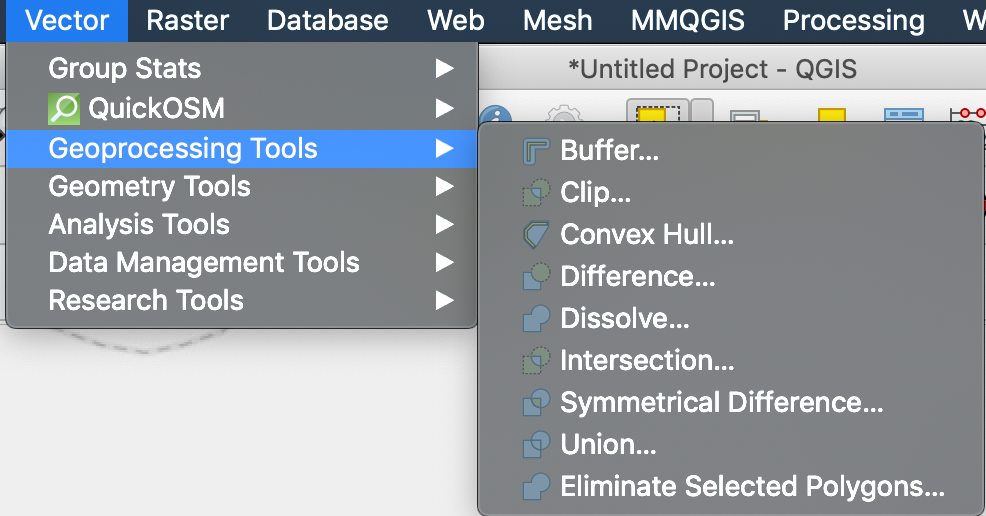

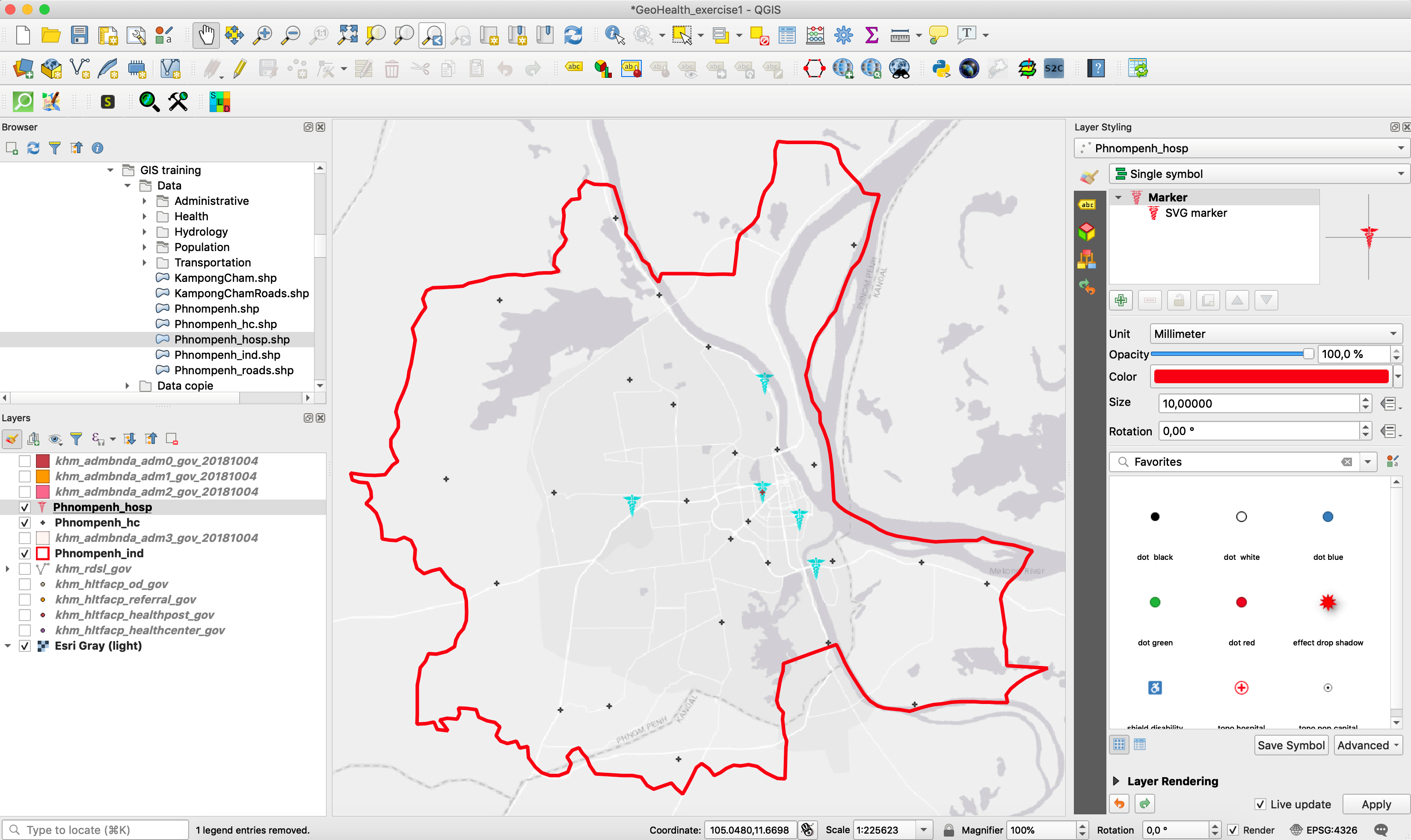
3.6 Creating a layer from GPS coordinates
Exercise: Create a shapefile from a csv file containing the longitude and latitude of Phnom Penh hospitals (as referred in OpenStreetMap).
-
-
- Open the Data Source Manager , choose the “Delimited Text” tab and browse to your csv file: Hospitals_OSM_PhnomPenh.csv
- Precise the file format (here, we use custom delimiters and check Comma) -> the table should be readable in the “Sample Data” box
- Precise the geometry: check “Point coordinates” and indicate the X and Y fields
- Precise the CRS of these points
- Press “Add”
- Save these imported points as a shapefile: right-click on the name of the imported file, choose Export / Save features as…
- Open the Data Source Manager
-
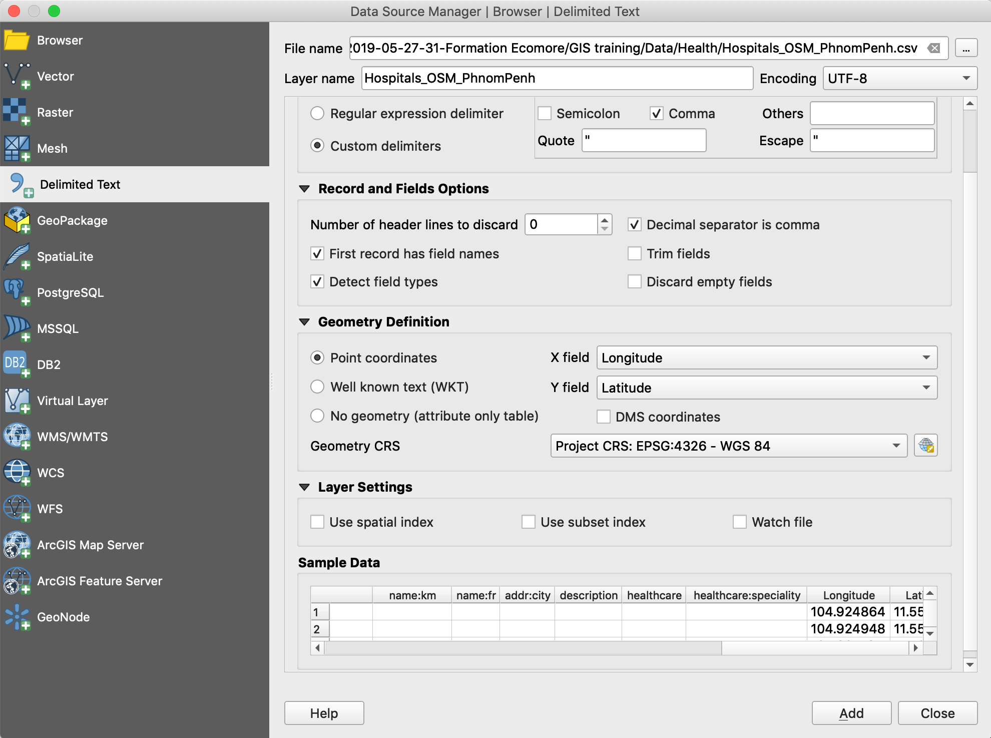
3.7 Creating buffer zones (buffers)
For the creation of buffer zones, we need a CRS in meters.
Exercise: Create buffers zones around health facilities
-
-
- Add the hospital layer to the canvas: khm_hltfacp_referral_gov.shp
- Check its CRS (-> Indian 60 / UTM zone 48N)
- Go to Vector menu / Geoprocessing Tools / Buffer…
- Choose Distance (for example here 10 kms), whether the overlapping buffers are dissolved or not, and a place to save your Buffered shapefile
- Run
-
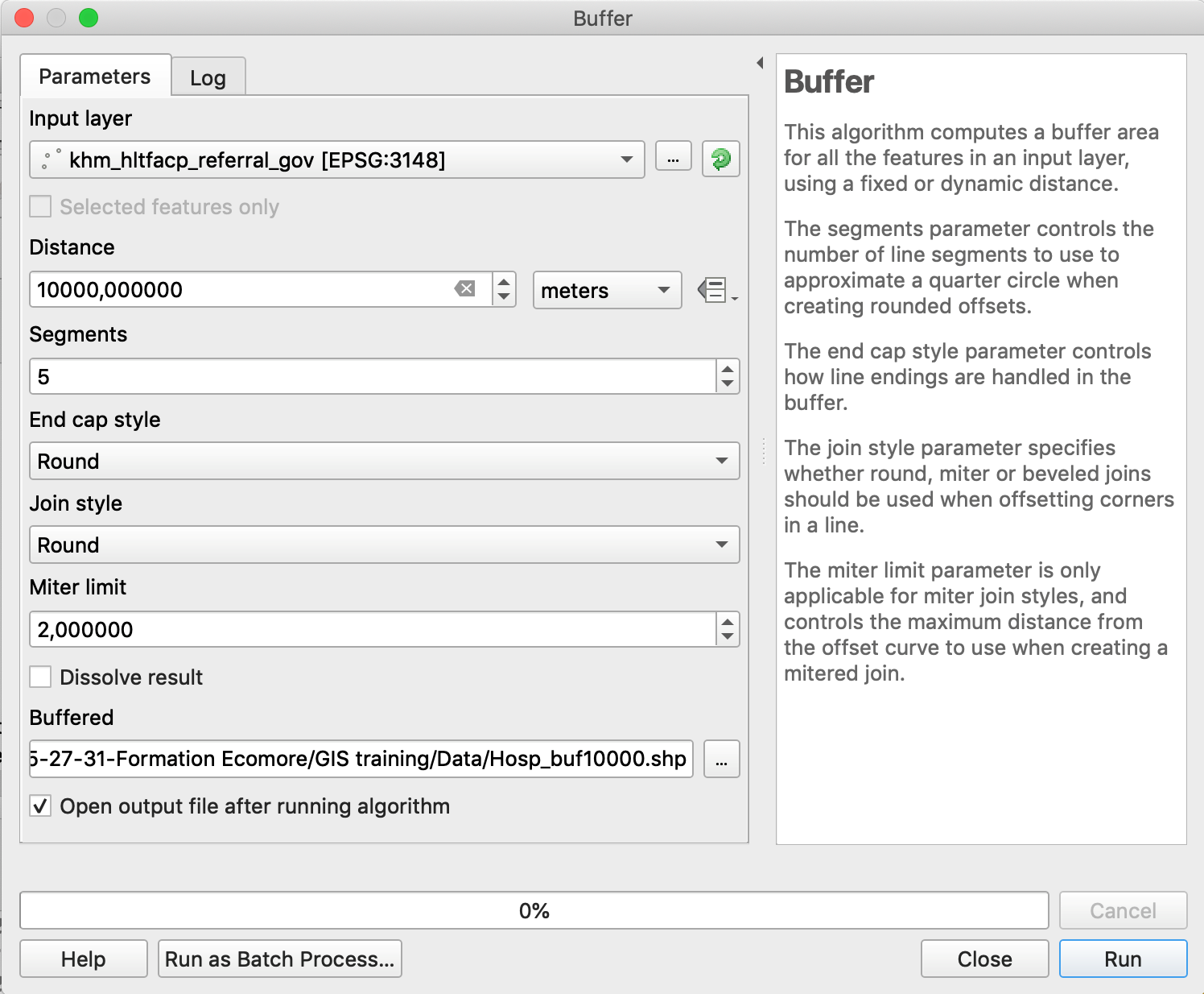
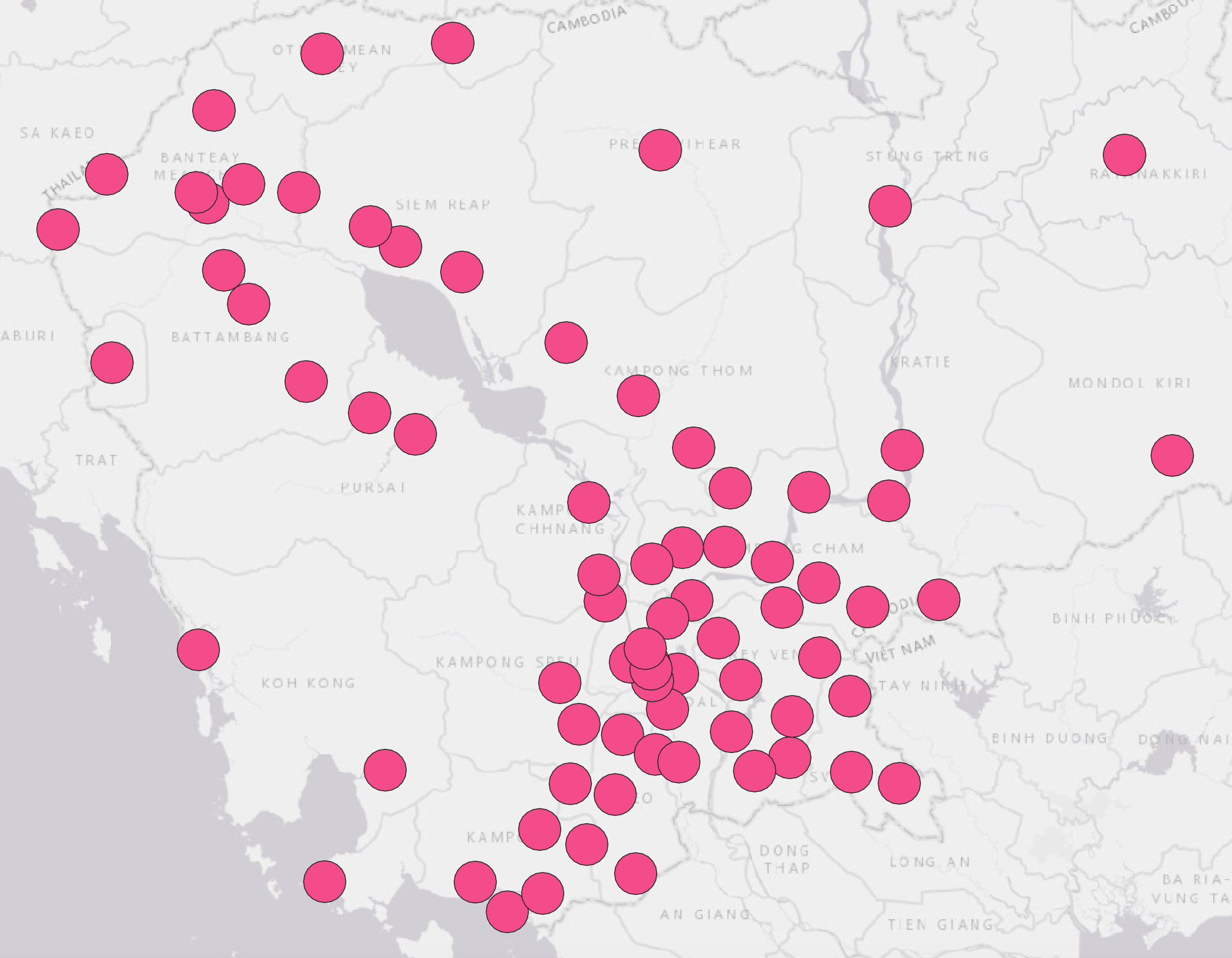
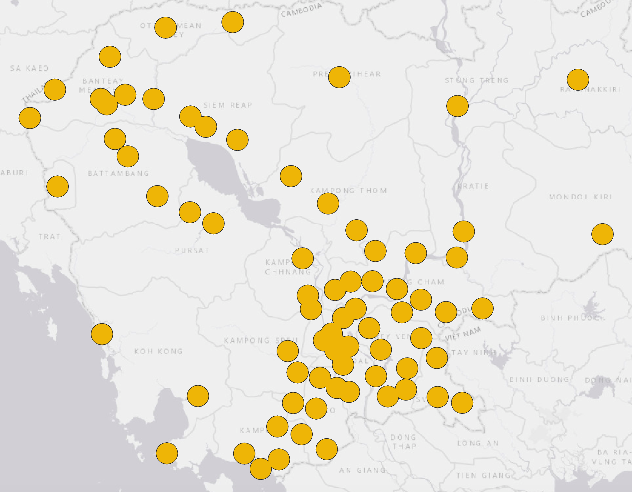
Note: Buffer zones can be created from any type of vector file (points / lines / polygons). The buffer zones will always be polygons.
3.8 Calculating distances between points (distance matrices)
A dedicated QGIS function allows you to directly calculate distances between two layers of points.
Exercise: Calculate the distances between the locations of the fictive patients (QGISfever.shp) and referral hospitals (khm_hltfacp_referral_gov.shp).
As with the creation of buffer zones, we need a CRS in meters to calculate distances.
-
-
- Go to Vector Menu / Analysis Tools / Distance Matrix…
- Choose the two point layers (containing n cases and m infrastructures)
- Choose the type of matrix:
- Linear distance matrix where all combinations will be in line (n*m lines)
- Standard distance matrix (with n rows and m columns)
- Specify the name and location of the output distance matrix. This matrix will be in.csv format
-
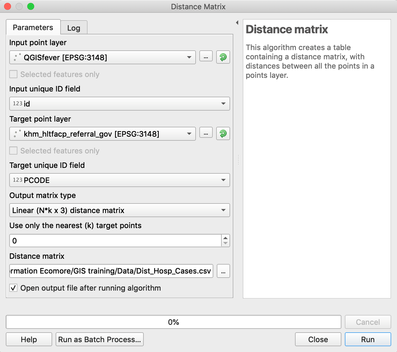
3.9 Calculating the number of points in a polygon
This function is very useful in epidemiology for calculating, for example, the number of cases per administrative unit.
Exercise: Calculate the number of “QGIS fever” cases in each district of Phnom Penh
-
-
- Reproject the district layer in the local projected CRS (Indian 60 / UTM zone 48N)
- Right-click on the name of the layer
- Export / Save Features As…
- Browse to your folder and give a new name indicated they are reprojected.
- Choose the new CRS
- OK
- Clip the district layer to the extent of Phnom Penh province:
- Go to Vector Menu / Geoprocessing Tools / Clip…
- Choose the district layer as the input layer
- Choose the Phnom Penh layer as the overlay layer
- Browse to your folder and give a name to the clipped layer
- Run
- Reproject the district layer in the local projected CRS (Indian 60 / UTM zone 48N)
-
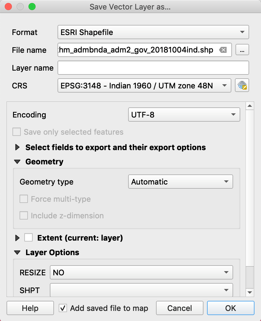
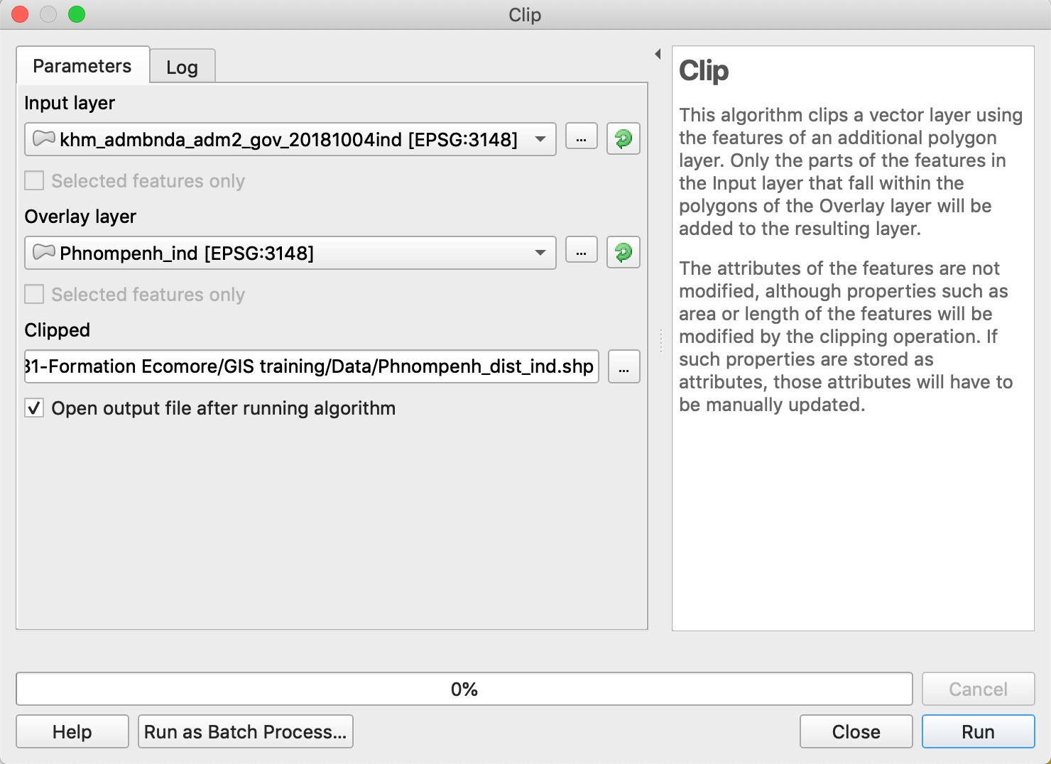
-
-
- Analysis Tools / Count Points in Polygon…
- Choose the district layer as Polygons
- Choose the QGIS fever layer as Points
- See the possible options to Weight fields (not used here)
- Specify a file name and folder for your output shapefile.
- Analysis Tools / Count Points in Polygon…
-
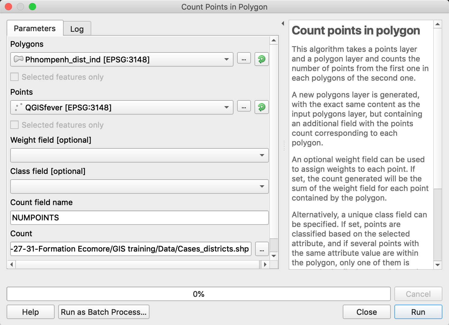
You can then represent the number of cases in each district by playing with the symbology
3.10 Exporting a layer to Google Earth
Note: This export could be useful when you want to exchange files with colleagues who do not know how to use a GIS, but who know the possibilities of Google Earth.
-
-
- Right-click on the name of your layer and choose Export / Save Features As…
- Choose the KML (Keyhole Markup Language) format
- Select the folder and name of your kml file to save
- OK
-
This kml file can be opened in Google Earth.
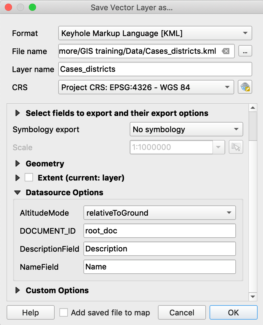
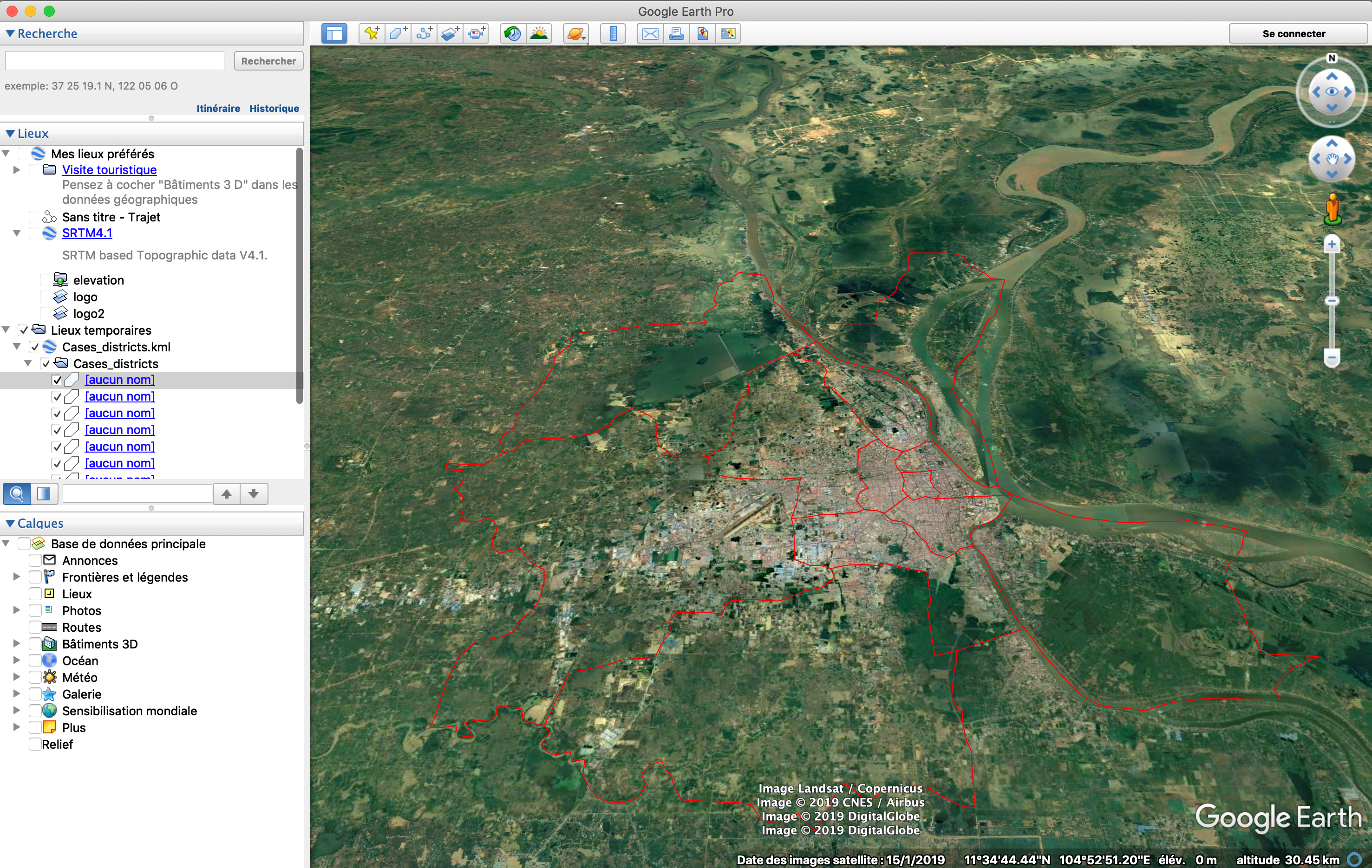
Tutorial QGIS – Discover
2. Creating a simple map and discovering the different toolbars
2.1 Downloading dataset
Cambodia administrative boundaries, divided in 4 levels:
-
-
- level 0: country,
- level 1: province / khaet and capital / reach thani,
- level 2: municipality, district,
- level 3: commune / khum, quarter / sangkat
-
These contours maps (shapefiles) are made available from the Humanitarian Data Exchange (HDX), provided by OCHA (United Nations Offices for the Coordination of Humanitarian Affairs: https://www.unocha.org/). These maps were originally produced by the Department of Geography of the Ministry of Land Management, Urbanization and Construction in 2008 and unofficially updated in 2014 according to sub-decrees on administrative modifications. They were provided by WFP - VAM unit Cambodia.
You can download these administrative boundaries, as zip folders, here:
https://data.humdata.org/dataset/cambodia-admin-level-0-international-boundaries
-
-
- khm_admbnda_adm0_gov_20181004.zip (127.0K)
- khm_admbnda_adm1_gov_20181004.zip (292.6K)
- khm_admbnda_adm2_gov_20181004.zip (589.2K)
- khm_admbnda_adm3_gov_20181004.zip (1.2M)
-
Population data:
Population data is available at these different levels from the Humanitarian Data Exchange (HDX) repository. It comes from the Commune database (CDB), provided by the Cambodia Ministry of Planning.
https://data.humdata.org/dataset/cambodia-population-statistics
Health Facility data:
The Humanitarian Data Exchange (HDX) repository provides a dataset on the location of health facilities (Referral Hospitals, Health Centers, Health Posts). These maps were originally produced by the Cambodia Ministry of Health (MoH).
https://data.humdata.org/dataset/cambodia-health
Transportation data:
The roads network is available from Humanitarian Data Exchange (HDX) repository. These maps were originally produced by the Cambodia Department of Geography of the Ministry of Land Management, Urbanization and Construction. They include: National road primary and secondary, Provincial road primary, Provincial and rural roads, Foot path, Cart track, Bridge line.
https://data.humdata.org/dataset/cambodia-roads
Hydrology data:
The hydrological network is available from Humanitarian Data Exchange (HDX) repository. These maps were originally produced by the Cambodia Department of Geography of the Ministry of Land Management, Urbanization and Construction. They include: rivers (“Non-Perenial/Intermittent/Fluctuating” and “Perennial/Permanent”), lakes
https://data.humdata.org/dataset/cambodia-water-courses-0
Digital Elevation Model (DEM)
The SRTM (Shuttle Radar Topography Mission) is a free DEM provided by NASA and NGA (formerly NIMA). Space Shuttle Endeavour (STS-99) collected these altimetry data during an 11-day mission in February 2000 at an altitude of 233 km using radar interferometry. The SRTM covers nearly 80% of the land area from 56° South latitude to 60° North latitude. Spatial resolution is approximately 30 meters on the line of the Equator.
The SRTM data can be downloaded here: http://srtm.csi.cgiar.org
2.2 Creating a project
QGIS starts with an untitled project but displays in the canvas the list of recent projects. By double-clicking on one of these recent projects, QGIS will quickly open it.
-
-
- You can start by saving your future project (file extension .qgz) :
-
In Menu Project -> Save as…
or by using the File Toolbar![]()
Note: Remember to frequently save your project!
2.3 Adding a vector layer
Note: Vector layers can be points, polylines or polygons.
-
-
- Add the four levels of Cambodian administrative layers (provinces, districts, communes) to the project:
-
- khm_admbnda_adm0_gov_20181004.shp (country)
- khm_admbnda_adm0_gov_20181004.shp (provinces)
- khm_admbnda_adm0_gov_20181004.shp (districts)
- khm_admbnda_adm0_gov_20181004.shp (communes)
-
- Add the four levels of Cambodian administrative layers (provinces, districts, communes) to the project:
-
There are several ways to add data to the project
- By using the Data Source Manager
- Open the Data Source Mangager by clicking on its icon in the Data Source Manager Toolbar
- Select the type of data to open : Vector / Raster / Delimited Text (csv) / etc.
- Browse to your file
- Click on Add button
- By using the Browser panel
- Find the .shp files in your folders
- Double-click the .shp files directly or drag and drop it to the map canvas
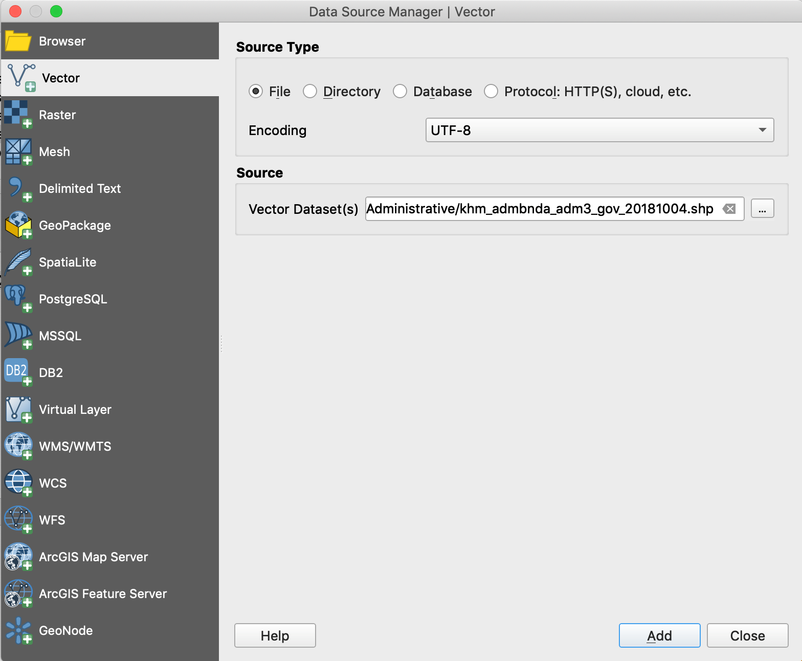
- By directly dragging and dropping the .shp files from your browser to QGIS
Note: You can select and open several files together with Ctrl or Shift keys.
Note: You can drag and drop layers in the table of contents to modify the order of appearance of the layers
2.4 Adding a basemap
QGIS 3 makes it very easy to add background maps (OpenStreetMap, Bing, MapBox, Google, etc.). Of course, this requires Internet connection.
Examples of basemap from different providers:
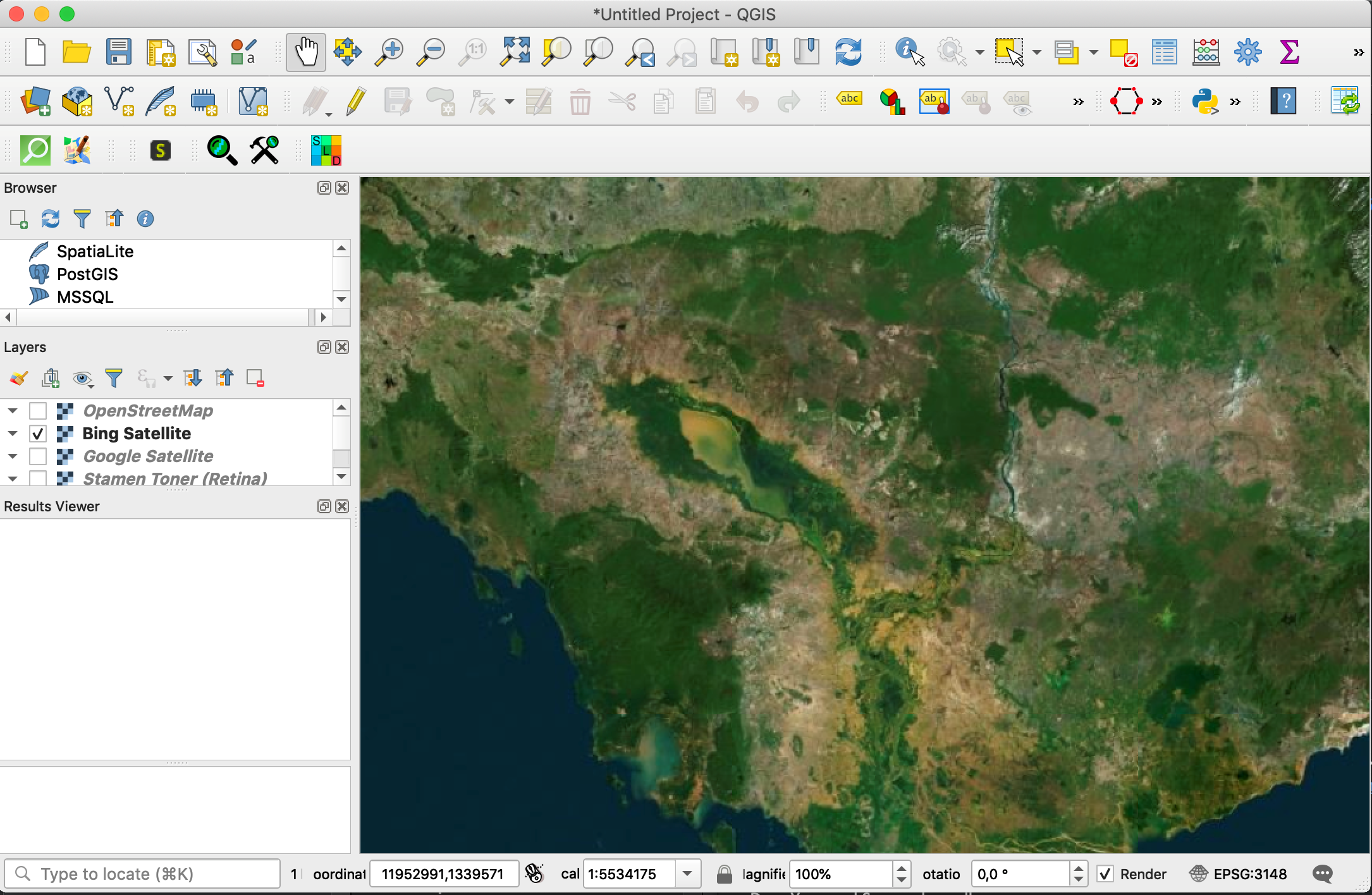
Microsoft Bing Satelitte basemap
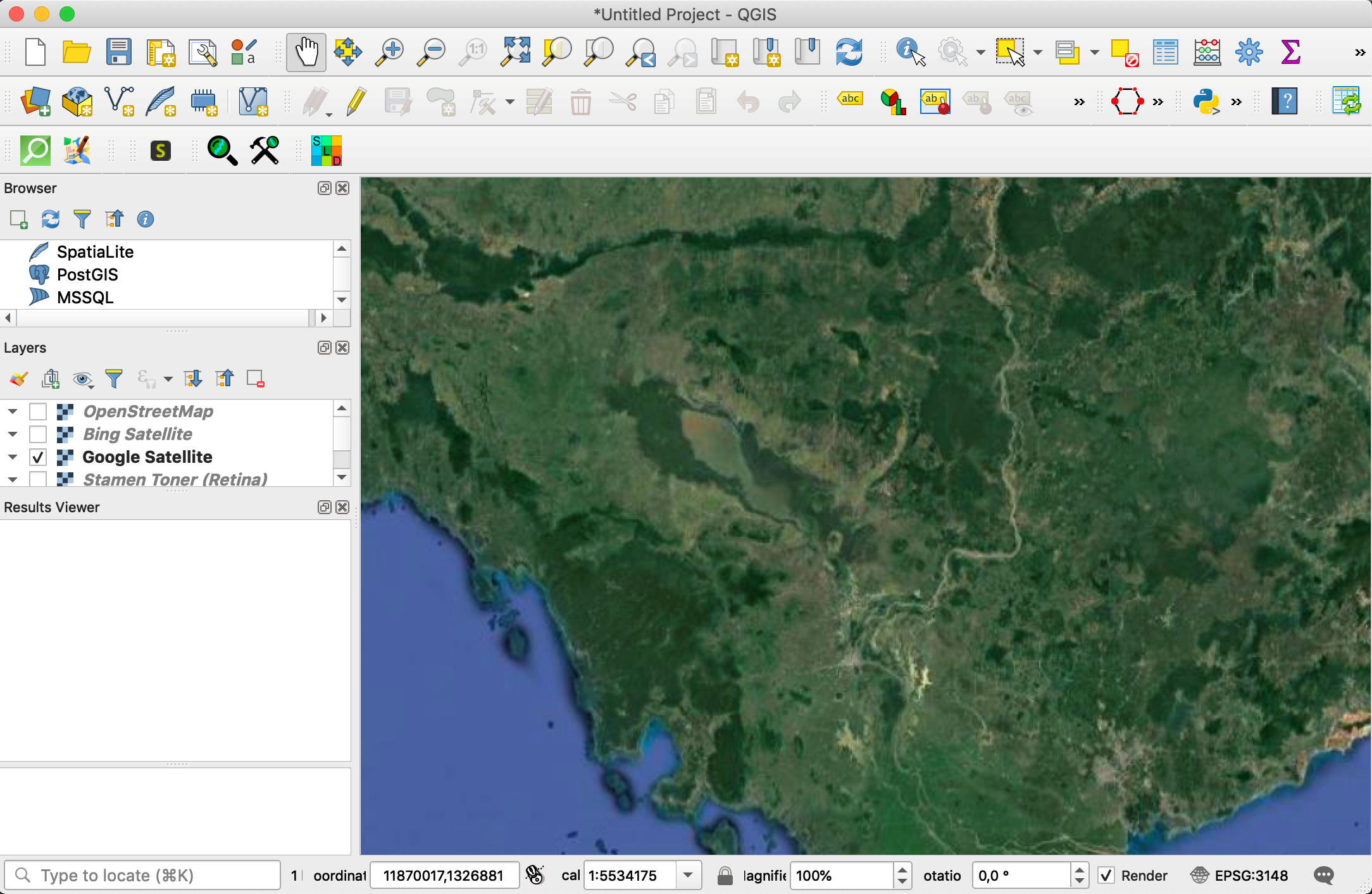
Google Satelitte basemap
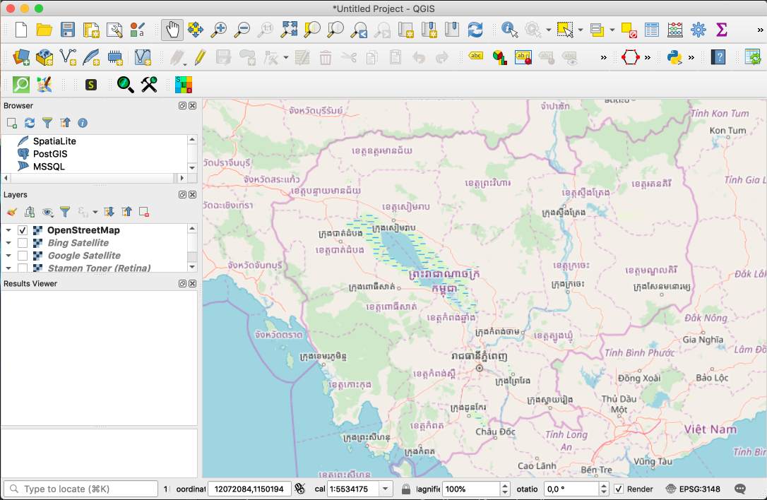
OpenStreetMap basemap
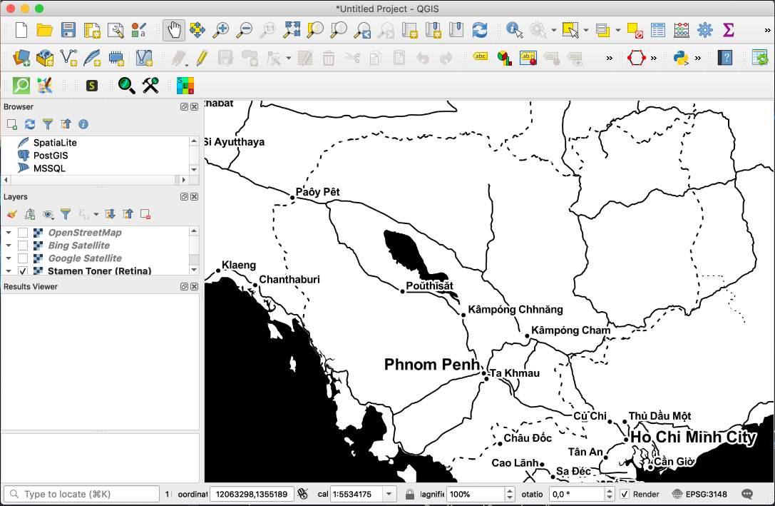
Stamen Toner basemap
There are several ways to add basemaps to QGIS:
- By using the Browser panel:
-
- In the Browser panel, go to XYZ Tiles and double click on OpenStreetMap
- By using a dedicated plugin:
You can also get a large list of basemaps using the QuickMapServices plugin:
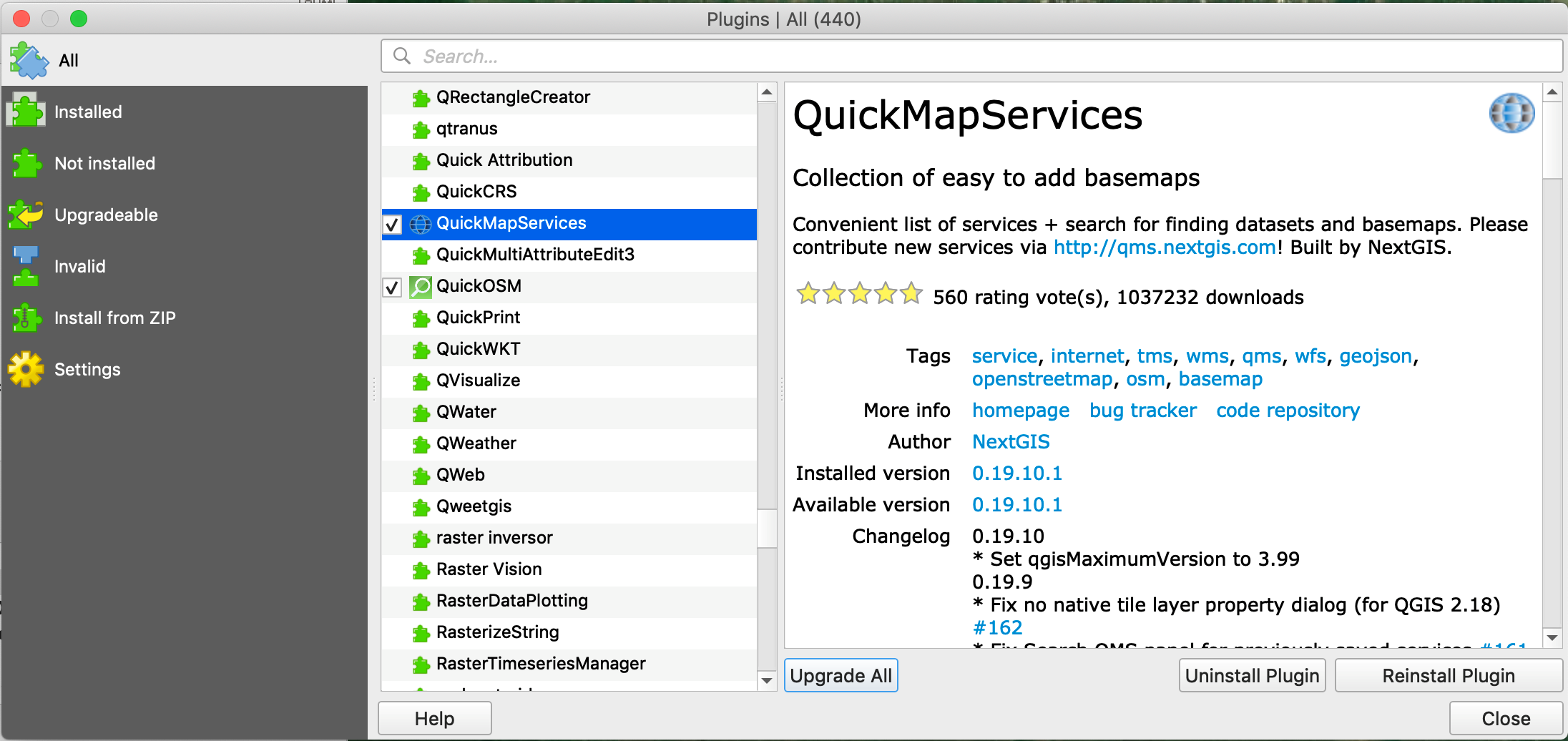
-
- Install QuickMapServices plugin by opening the Plugin Manager
- Menu Plugins / Install and Manage Plugins…
- Search for QuickMapServices (you can type “Quick” in the Search window)
-> this plugin will be installed in the Web Menu
-
- Go to Menu Web / QuickMapServices
- Select the basemap you would like to display
QuickMap Services Plugin offers also precise settings for the visibility of the maps in the plugin, for getting more maps or for the download timeout.
-
- In the QuickMapServices Menu, go to Settings
- Go to the More Services tab
- Click on “Get contributed pack” to obtain more maps
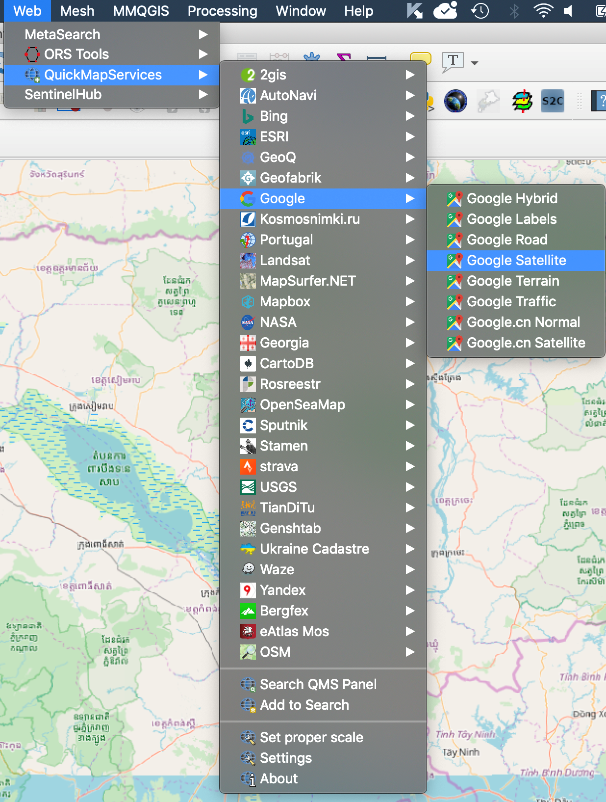
Note: do not open too many basemaps since it will require internet
Alternatively, you can use the OpenLayers Plugin that will be also installed in the Web Menu but it offers less possibilities.
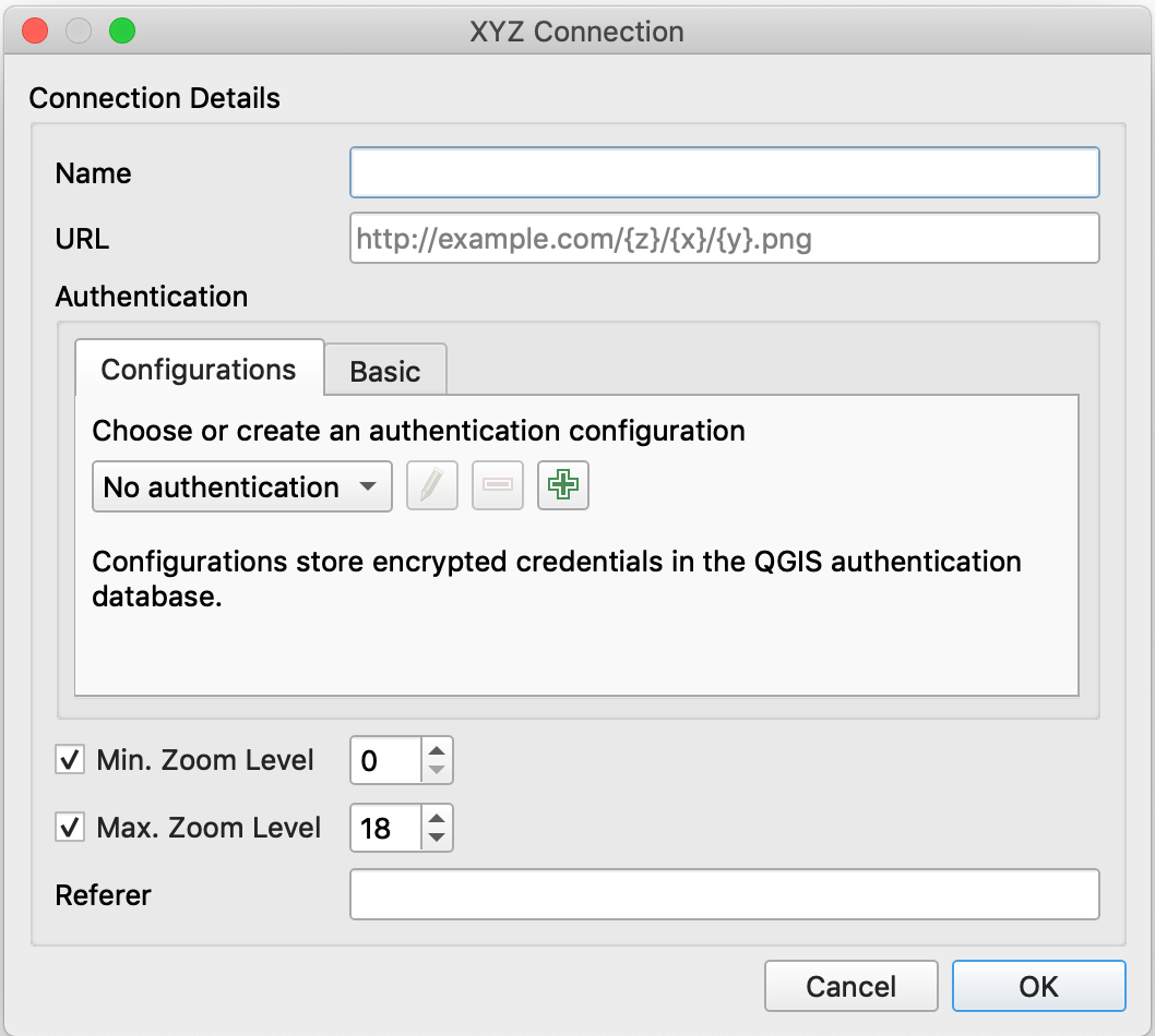
It is possible to add more basemaps in the XYZ Tiles Browser by connecting to other tile services
See: https://opengislab.com/blog/2018/4/15/add-basemaps-in-qgis-30
-
-
- Right-click on XYZ Tiles in the Browser Panel
- Select New Connection…
- Enter the name and URL of basemap
-
Example for Google Satellite: https://mt1.google.com/vt/lyrs=s&x=%7Bx%7D&y=%7By%7D&z=%7Bz%7D
There is also the possibility to use a Python script to directly add several basemaps to the Browser:
-
- Copy the script here: https://raw.githubusercontent.com/klakar/QGIS_resources/master/collections/Geosupportsystem/python/qgis_basemaps.py
- Open the Python Console in the Plugins Menu / Python Console
- Paste the script and Run Python
- It will automatically update the liste of XYZ tiles (Thanks to the contributors of this nice Python script!).
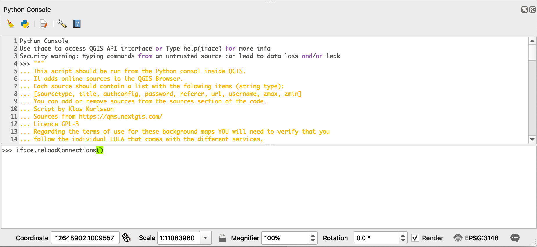
2.5 Moving around the map
Map Navigation toolbar ![]()
Test the different tools:
-
-
- Pan map,
- Pan map to selection,
- Zooming: Zoom In, Zoom Out, Zoom to Native Resolution, Zoom Full, Zoom to Selection, Zoom to Layer, Zoom Last, Zoom Next,
- Refresh
-
Control the scale and the geographic coordinates of the map:
A specific scale can be given on the bottom right side of the window. ![]()
Also you can visualize the coordinates of the location of the mouse over the main window.![]()
2.6 Selecting and getting information on attributes
Attribute toolbar ![]()
Test the different tools:
-
- Identify features: First select a layer in the Layer Panel and then click on the object to display its information.
- Select Features: First select a layer in the Layer Panel, then choose between:
-
- Select Feature(s),
- Select Features by Polygon / by Freehand / by Radius
- Select Features by Value
- Deselect Features from all layers.
-
- Open Attribute Table: First select a layer in the Layer Panel and then click on this icon to display its table.
- Open Field Calculator
- Open Processing Toolbox
- Show Statistical summary
- Measure Line / Area / Angle
- Show Map Tips
- New Bookmark
- Show Bookmark
- Annotation: Text / Form / HTML / SVG / Move.
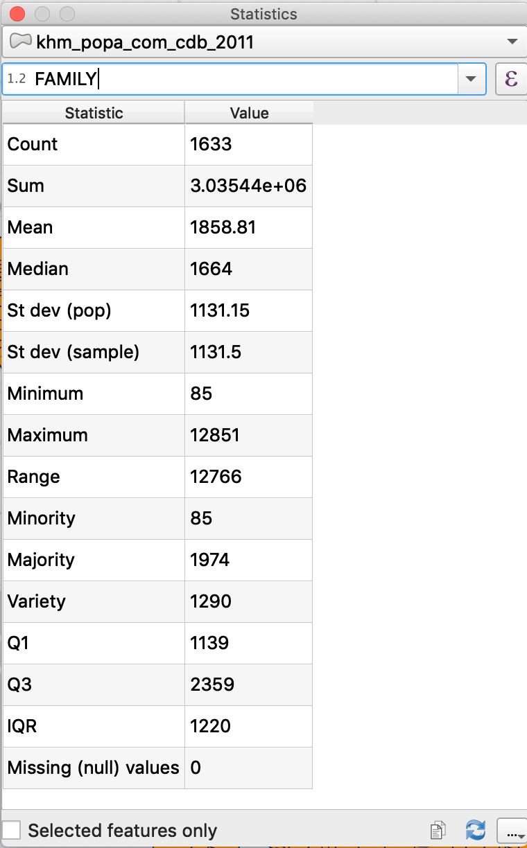
2.7 Adjusting the symbology
-
- Choose khm_admbnda_adm1_gov_20181004.shp
- Double click on the name of the layer to open the Layer properties window
- Choose the Symbology tab
- Here you will be able to select Single symbol / Categorized / Graduated / Rule-based / Point displacement
- Choose Categorized, choose the HRName column and click on Classify
- See the different options, with colors, and layer rendering
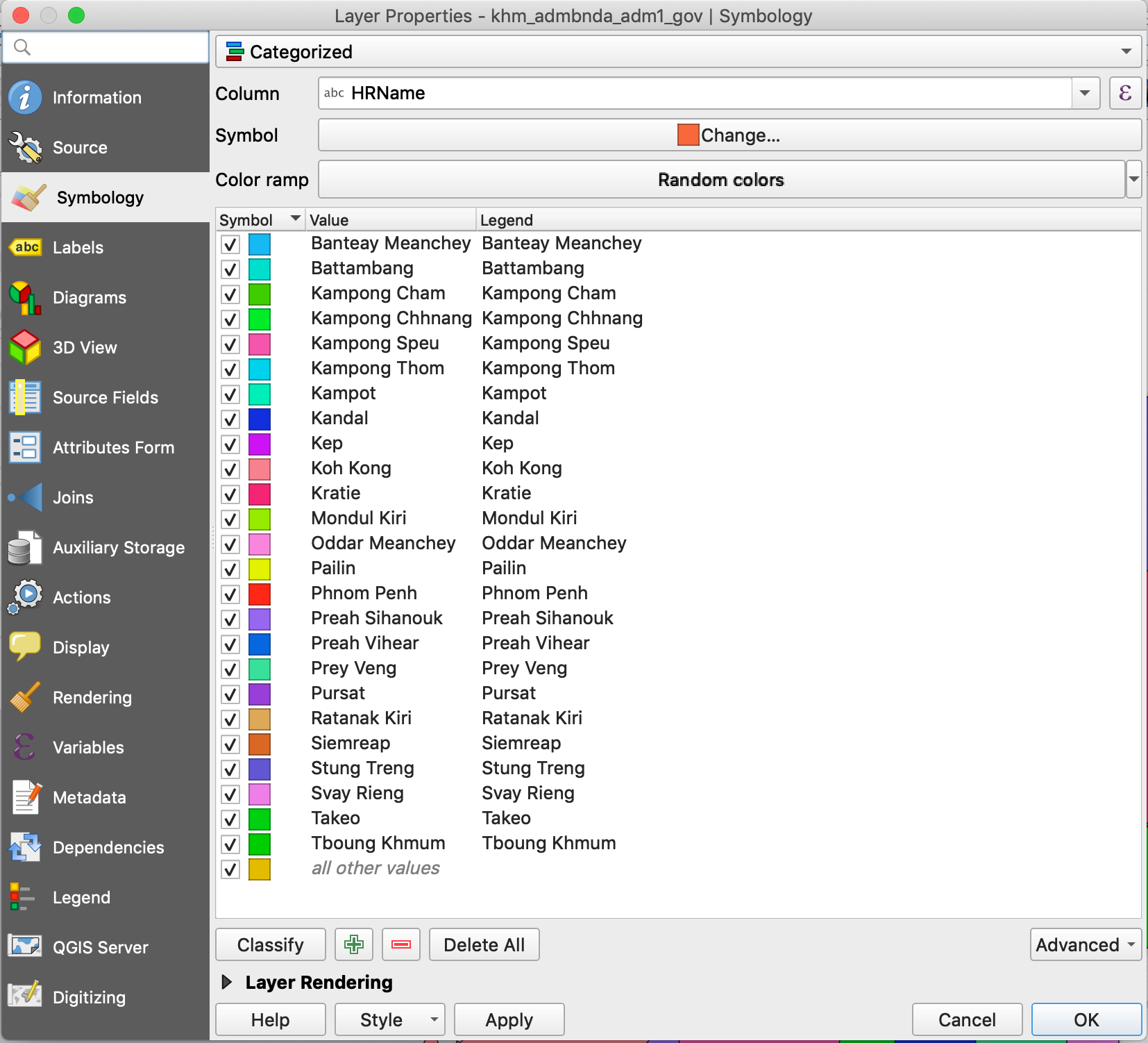
Alternatively, you can open the Layer Styling Panel with the shortcut in the top of the Layers Panel.
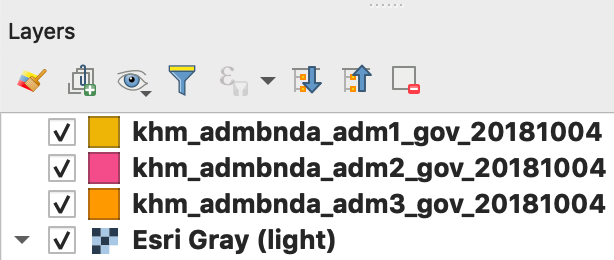
2.8 Choosing layer units
You may like to display your map either in “Degrees, Minutes, Seconds”, in “Decimal degrees” or in Meters.
-
- Go to Project / Properties / Tab General
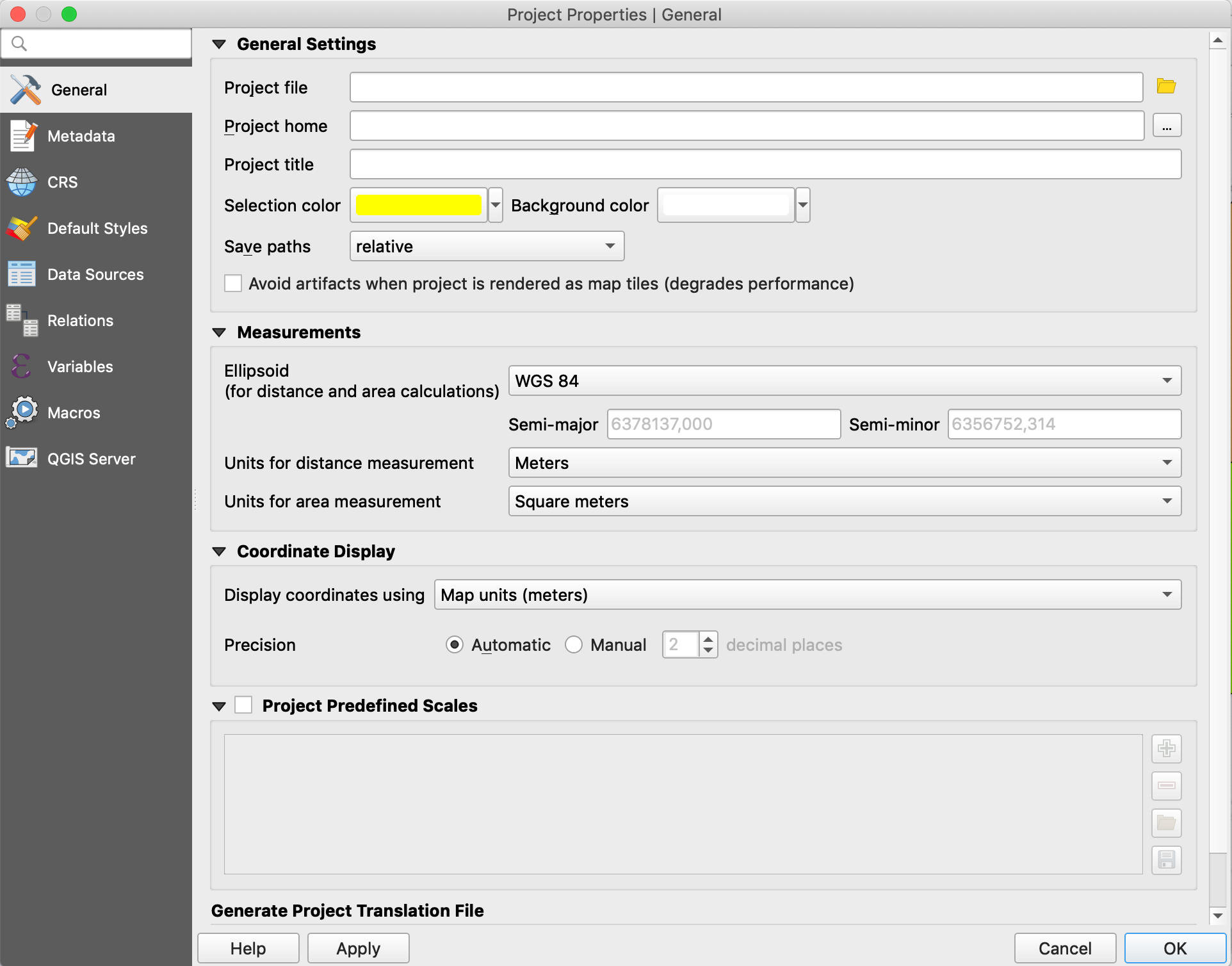
2.9 Using Projections
QGIS allows to define a Coordinate Reference System (CRS) by default or for the whole project, for layers without predefined CRS. It also allows to define customized CRS and allows the projection of vector layers on the fly.

Notes: Layers should be in the same CRS to allow geoprocessing. Indeed, we will have to check and pay attention to the CRS of each layer when using them for spatial analyses. However QGIS can display layers with different CRS on the same extent.
Layers should use a projection in meters, when calculating distances or buffers.
QGIS manages approximately 2,700 CRS.
For this training using data from Cambodia, we will use the following projections:
-
-
- Geographic CRS (in decimal degrees): WGS 84 (EPSG:4326)
-
-> This CRS has a worldwide coverage and is used for Google and OpenStreetMap data.
-
-
- Global projected CRS (in meters): WGS 84 / UTM zone 48N (EPSG:32648)
- Local projected CRS (in meters): Indian 60 / UTM zone 48N (EPSG:3148)
-
Specify the CRS of a layer:
-
-
- Double click on the name of the layer to open the Layer properties window
- Choose the Source tab
- Click on the Select CRS button
- Choose the desired projection from the top list if it appears among those recently used, otherwise from the bottom list.
- Use the filter if the desired projection does not appear in the top list.
- You can save the layer with a new projection: this is the way to reproject a layer.
-
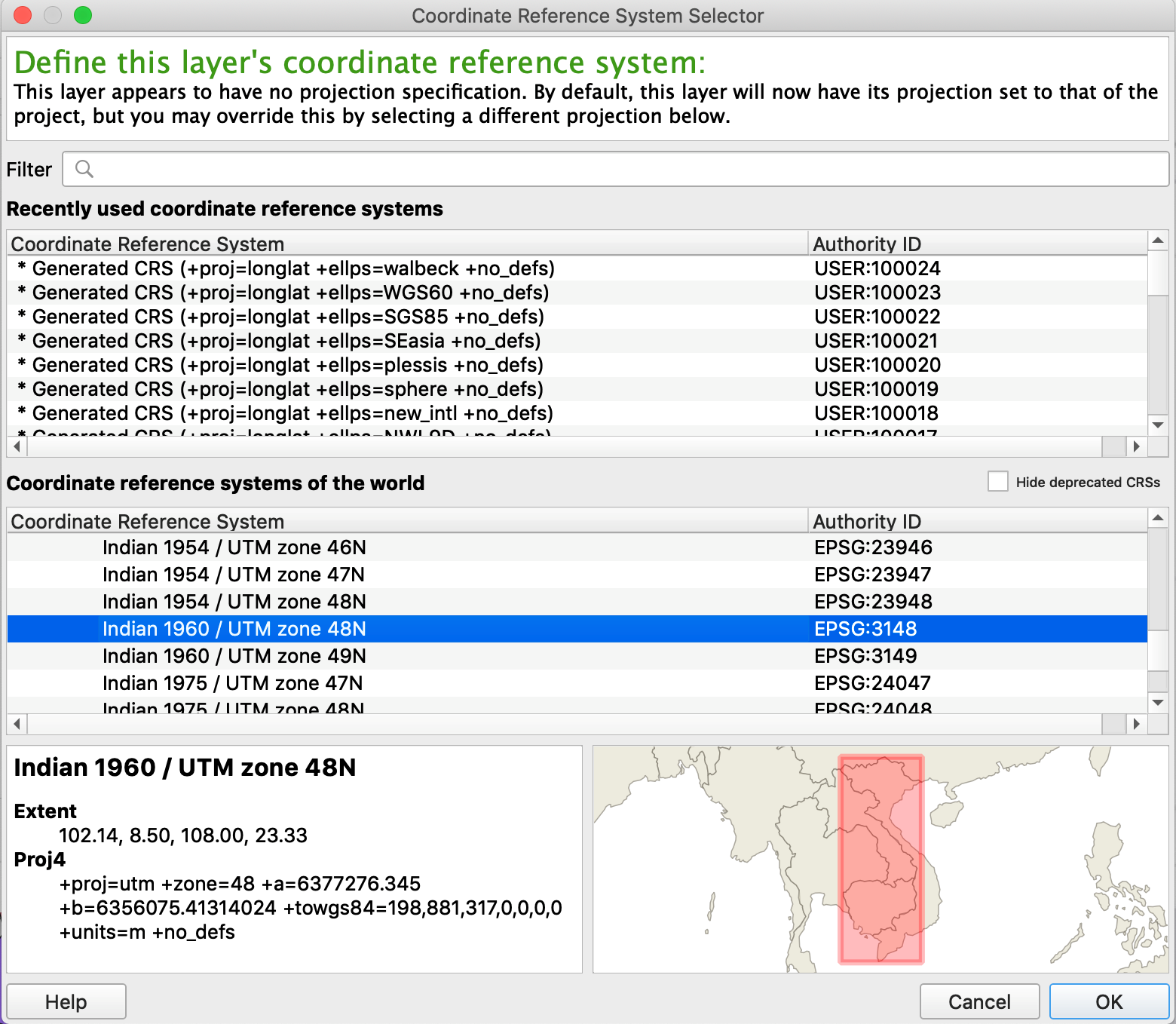
Exercise:
-
- Check the CRS of your administrative files (WGS 84).
- Reproject them into Local projected CRS (Indian 60 / UTM zone 48N):
- Right-click on the name of the layer
- Export / Save Features As…
- Browse to your folder and give a new name indicated they are reprojected.
- Choose the new CRS
- OK
Specify the SCR of a project:
-
- Go to Project / Properties
- Select the Coordinate Reference System (CRS) tab
- Choose the desired CRS
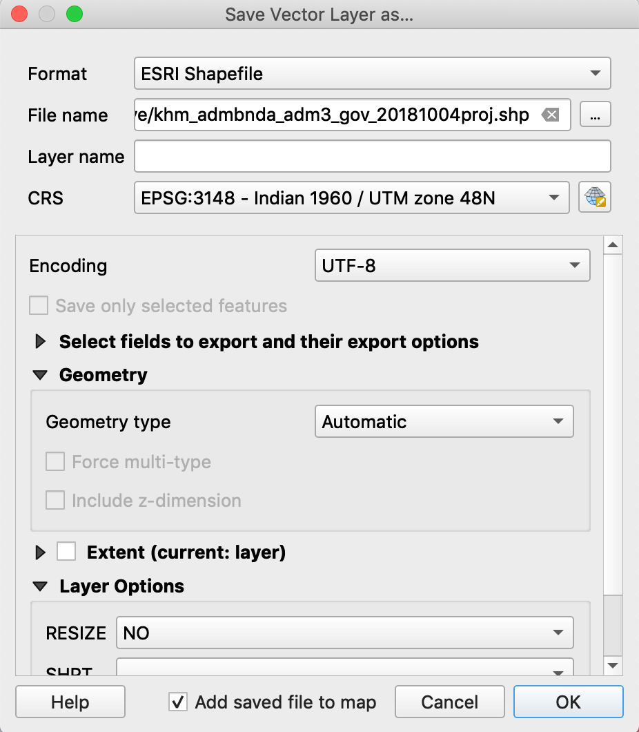
Tutorial QGIS – Installation
1. Installing and starting QGIS
1.1 Downloading and installing QGIS
- The latest version is QGIS 3.6, called Noosa and published on February 2019
- The latest Long Term Release (LTR) is QGIS 3.4, called Madeira and published on October 2018.
- Download from QGIS website:
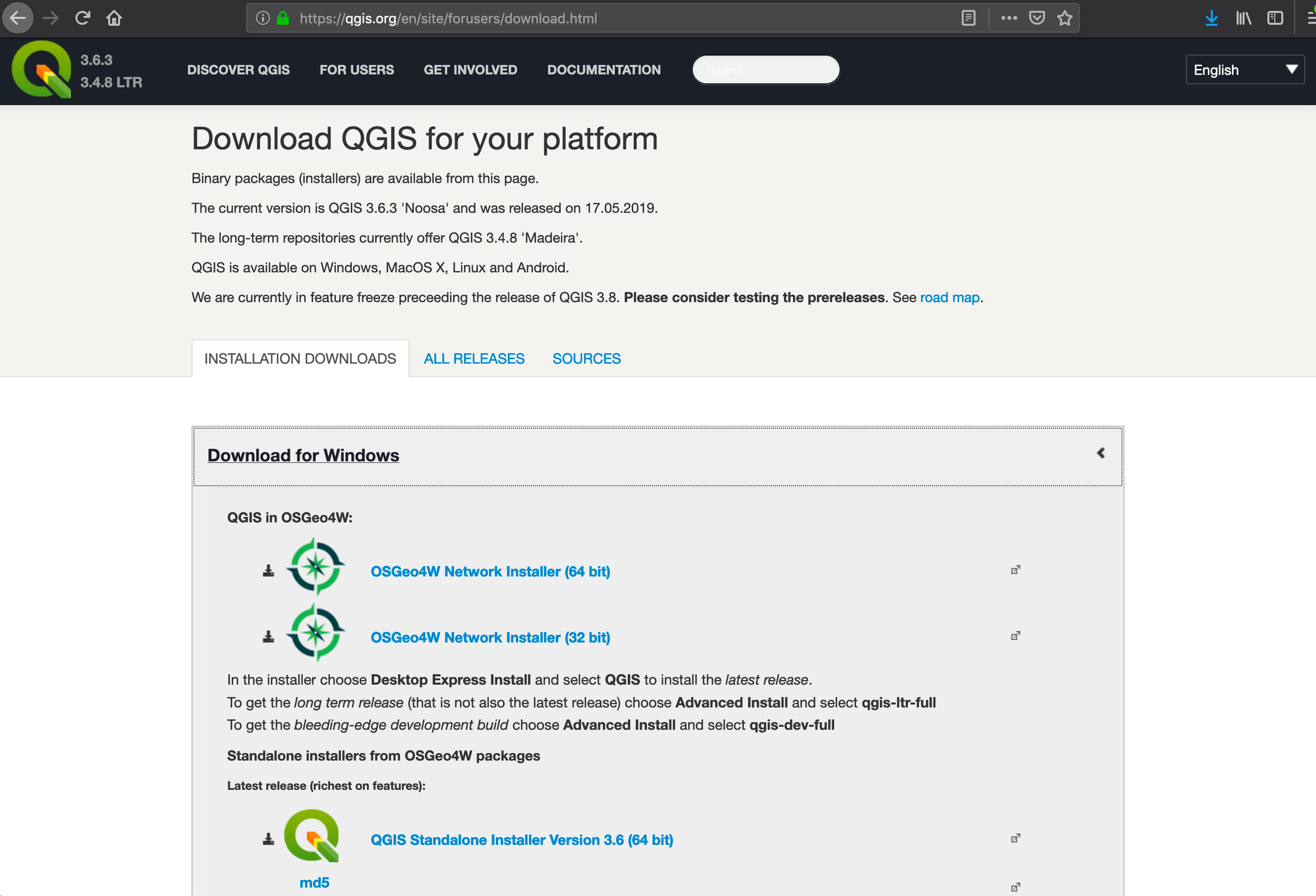
- The installation does not raise any particular difficulties

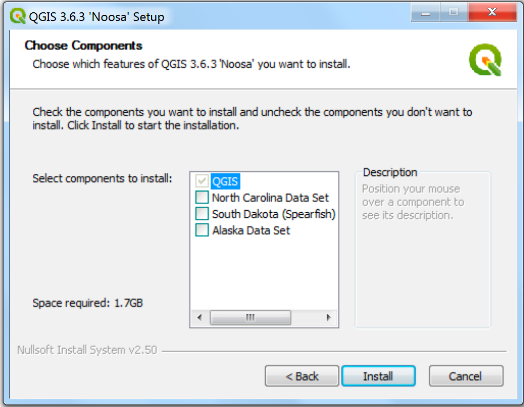
1.2 Starting QGIS
- Use the QGIS shortcut on desktop :
 QGIS Desktop 3.6.3
 - Or go to: Startup menu / All Programs / QGIS 3.6 / QGIS Desktop 3.6.3
The QGIS graphical interface is divided into 6 zones:
- Menu Bar
- Toolbars
- File browser
- Layers, Legends
- Map canvas
- Locator bar
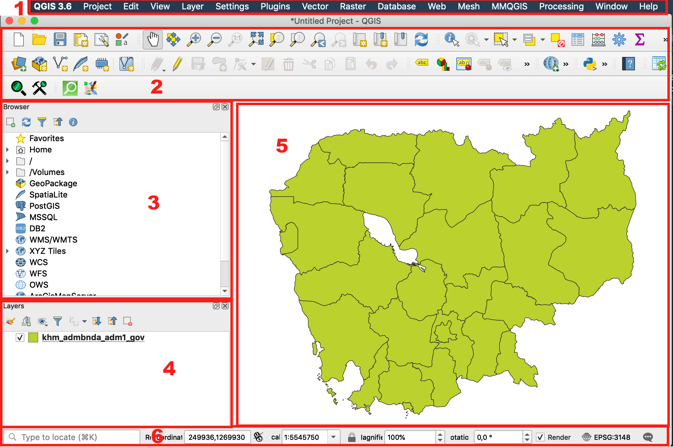
Note : The graphical user interface may appear differently depending on your operating system and configuration of toolbars.
The available toolbars depend on the installed plugins.
Panels and toolbars can be displayed or hidden by:
-
-
- right-clicking in the grey area of the toolbars to open the panel selection (top list) and toolbar selection (bottom list).
- Going to the View Menu / Panels or View / Toolbars
-
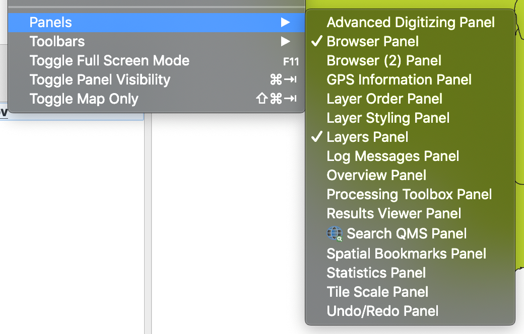
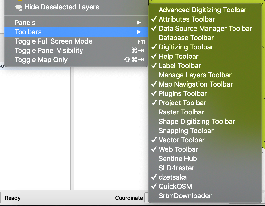
1.3 Specifying QGIS Options
QGIS is developed in English but the GUI can be used in different languages according to the available translations. It is easy to switch from one language to another one:
- Go to the Preferences / General tab
- Select Override system locale if necessary and chose the translation
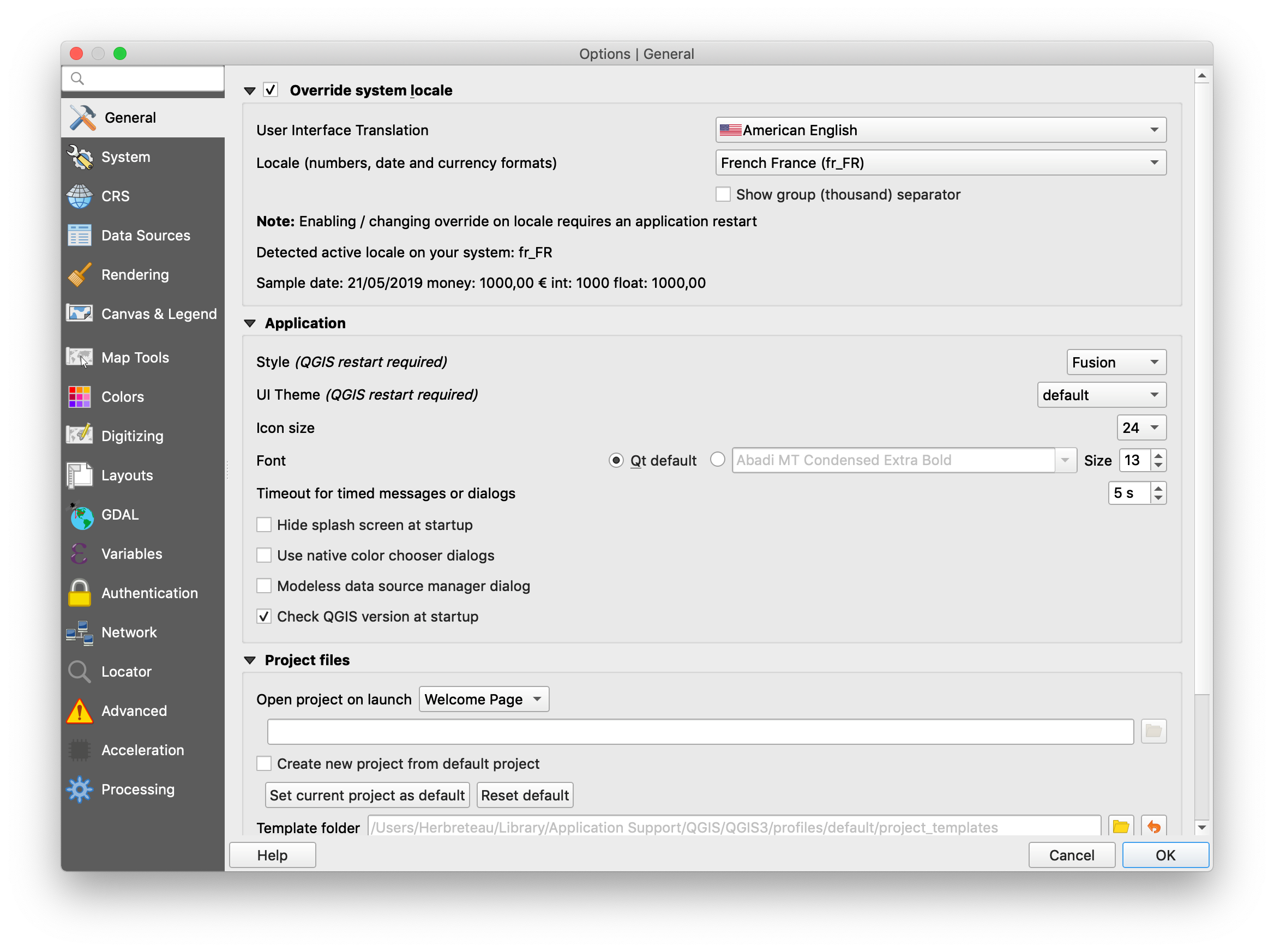
- Verify also the units and date formats in the Locale list.
About
The GeoHealth Team conducts research in South-East Asia on the climate, environmental and social factors that drive the spatiotemporal dynamics of diseases to improve modelling and surveillance. The team also develops the use of data from Earth-observation satellites to build environmental monitoring systems that can help health managers to detect early signals and understand health risks.
The team is mainly based at the KHmer Earth OBServation (KHEOBS) Laboratory, a collaboration between the Institute of Technology of Cambodia (ITC) and the French National Research Institute for Sustainable Development (IRD) in Phnom Penh with interaction with the Espace-Dev colleagues in Montpellier (Maison de la Télédétection) and at La Réunion (SEAS-OI Station). KHEOBS is a laboratory dedicated to build capacities in remote sensing for environment and climate monitoring.
GeoHealth collaborates closely with several research institutes and health institutions in Cambodia (Cambodian CDC at the Ministry of Health and Institut Pasteur du Cambodge) and Thailand (Ministry of Public Health, Shoklo Malaria Research Unit (SMRU), Mahidol University).
Posts page

GeoHealth updated their status.
When this happens, it's usually because the owner only shared it with a small group of people, changed who can see it or it's been deleted.
GeoHealth updated their status.
When this happens, it's usually because the owner only shared it with a small group of people, changed who can see it or it's been deleted.
GeoHealth updated their status.
When this happens, it's usually because the owner only shared it with a small group of people, changed who can see it or it's been deleted.

GeoHealth
United in Science 2023, by the World Meteorological Organization (WMO)
A multi-organization high-level compilation of the latest weather-, climate and water-related sciences and services for sustainable development, including services for health.
Conclusion: "Enhancing transdisciplinary collaboration between the weather, climate, water and health science communities will be crucial in development of climate services for the health sector"
GeoHealth updated their status.
When this happens, it's usually because the owner only shared it with a small group of people, changed who can see it or it's been deleted.

GeoHealth
In a study of 20 years of data from the NASA/German GRACE and GRACE-FO satellites, two NASA scientists confirmed that major droughts and pluvials — periods of excessive precipitation and water storage on the landscape — have been occurring more often. They also found that the worldwide intensity of these extreme wet and dry events – a metric that combines extent, duration, and severity — is closely linked to global warming.
NASA Scientific Visualization Studio - Water Cycle Extremes: Droughts and Pluvials
This visualization shows extremes of the water cycle — droughts and pluvials — over a twenty-year period (2002-2021) based on observations from the GRACE and GRACE-FO satellites. Dry events are shown as red spheres and wet events as blue spheres, with earlier years being shown as lighter shades ...
GeoHealth updated their status.
When this happens, it's usually because the owner only shared it with a small group of people, changed who can see it or it's been deleted.
GeoHealth updated their status.
When this happens, it's usually because the owner only shared it with a small group of people, changed who can see it or it's been deleted.

GeoHealth
In a just published litterature "review of Importance of Weather and Environmental Variables in Agent-Based Arbovirus Models", Pascoe et al. conclude that "climatic and environmental factors may influence the arbovirus disease outbreak, transmission, and surveillance. (...) it is crucial to consider the influence of climatic and environmental factors, especially in Africa, where there are limited studies exploring this phenomenon."
Review of Importance of Weather and Environmental Variables in Agent-Based Arbovirus Models
The study sought to review the works of literature on agent-based modeling and the influence of climatic and environmental factors on disease outbreak, transmission, and surveillance. Thus, drawing the influence of environmental variables such as vegetation index, households, mosquito habitats, bree...

GeoHealth
Nicely designed world maps of mortality rates of communicable and non-communicable diseases in 2019, proposed by Cartoprodig (UMR PRODIG) in their great maps repository (over 400 maps)
www.cartoprodig.cnrs.fr/carte/taux-de-mortalite-par-cause-de-maladies-non-transmissibles-du-total-2019-6/
www.cartoprodig.cnrs.fr/carte/taux-de-mortalite-par-cause-de-maladies-transmissibles-maternelle-perinatale-ou-nutritionnelle-du-total-2019-6/
Télécharger (JPG pour écran, 1,3 Mo) Télécharger (PDF pour impression, 3,1 Mo)Tous les contenus de ce site internet sont publiés sous licence Creative Commons Paternité, pas d’usage commercial, pas de modification.Pour en savoir plus, consultez le site officiel. Source à indiquer : © cart...
Special Issue on “Remote Sensing for Health: from Fine-scale Investigations towards Early-warning Systems” in the Remote Sensing Journal (IF 5.3), with 11 articles published in 2020
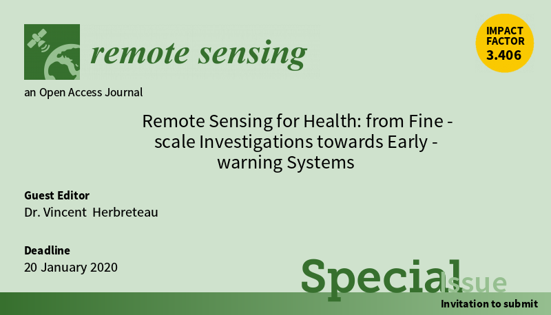
Home
Contact
[si-contact-form form=’1′]
Réunion
Carte de la Réunion by Stamen
[mapsmarker layer=”1″]