
3. Using Vector Data
3.1 Downloading OpenStreetMap data
OpenStreetMap (OSM: www.openstreetmap.org) is an open-access geographic database of the World. You are free to use it for any purpose as long as you credit OpenStreetMap and its contributors.
The QuickOSM plugin, developed by Etienne Trimaille at 3Liz, is the easiest way to access OSM data, through the Overpass API. Users can directly request OSM features over a given extent, by defining the keys, values and boundaries in the Quick Query tab. Users can choose to act directly on the script to best configure their request after clicking on the “Show query” button.
- Install QuickOSM from the plugins manager
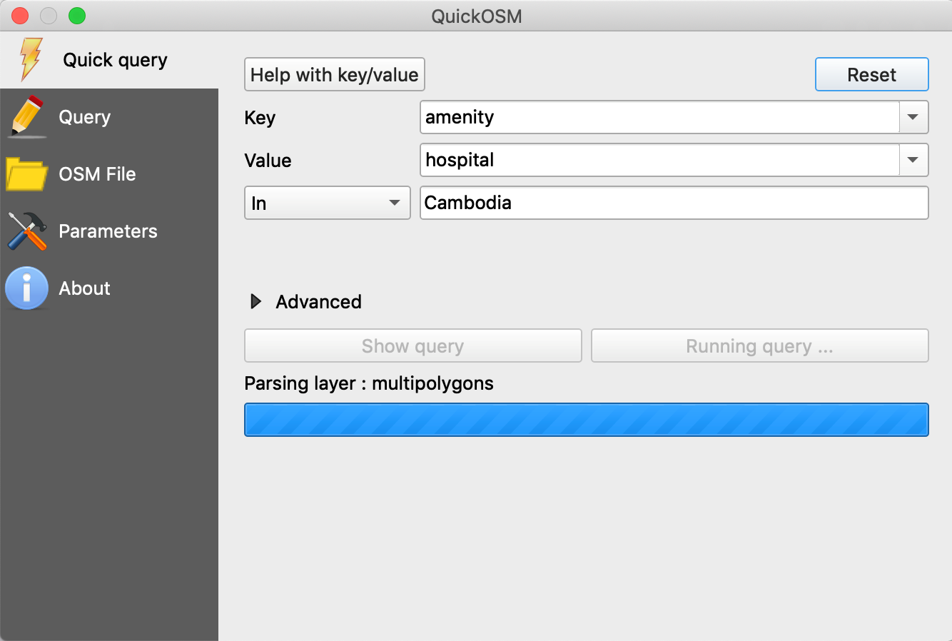
Exercise: Download the hospitals of Cambodia
- Go to Vector / QuickOSM / QuickOSM
- In the Quick query, choose:
- Key = amenity
- Value = hospital
- In = Cambodia
- Run query
- Data will be downloaded as polygon and points shapefiles
- In the “Advanced” list, you can choose the type of data to download (Node / Way / Relation / etc.) or increase the timeout if necessary
- Export the downloaded data as shapefile for further uses
Note: Clicking on the “Help with key/value” will directly open the Map Features page of the OSM wiki: https://wiki.openstreetmap.org/wiki/Mapfeatures
For administrative boundaries, check here the administrative levels by country: https://wiki.openstreetmap.org/wiki/Tag:boundary%3Dadministrative#10_admin_level_values_for_specific_countries
3.2 Joining a data table to a map
In this exercise, we will join the population data (khm_pop_2016_adm3_v2.csv) to the layer of communes khm_admbnda_adm3_gov_20181004.shp based on a common field.
- Add the layershp to the map
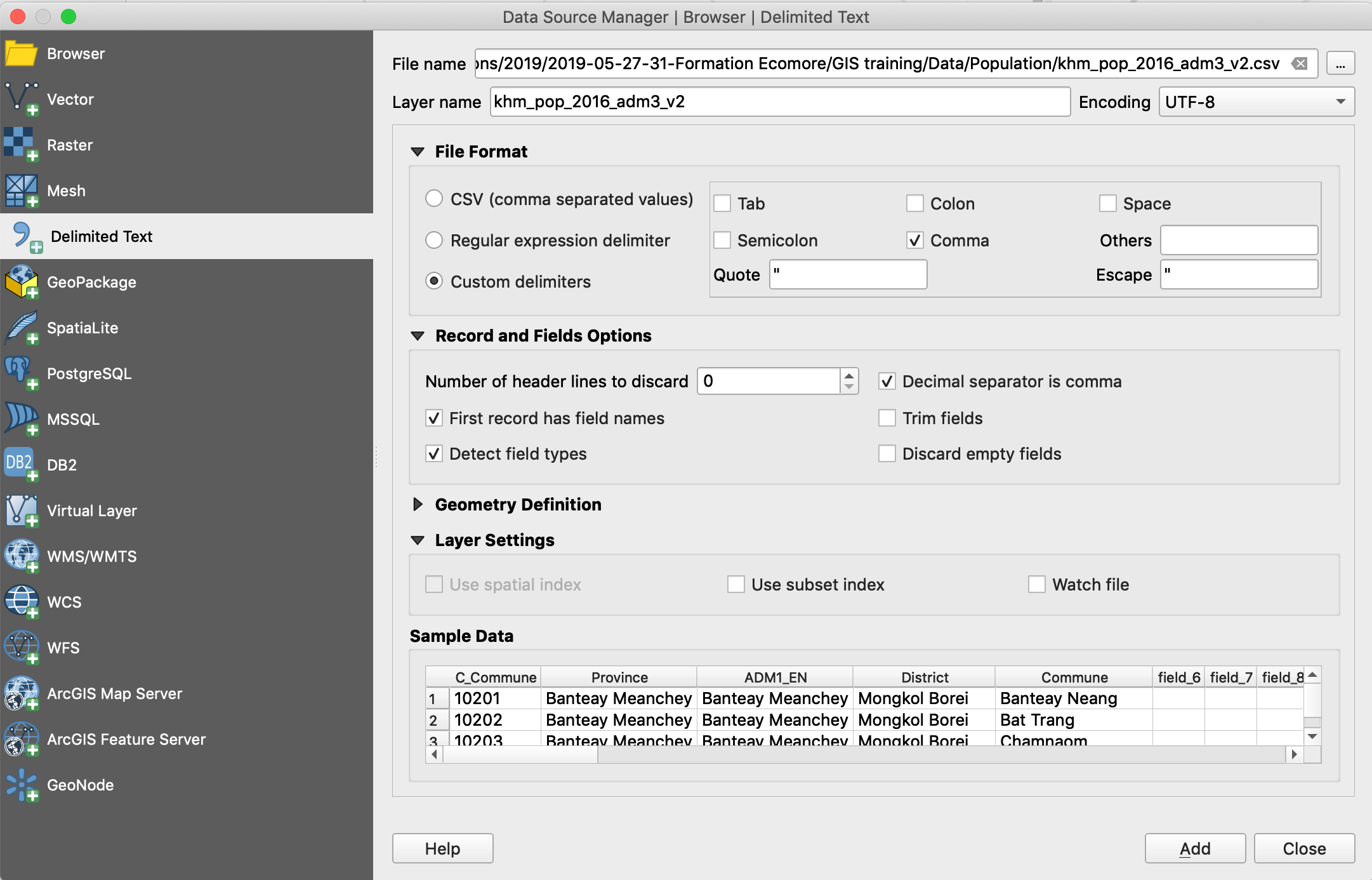
- Add the tablecsv the project. It cannot be directly added by double-click because settings should be carefully checked to ensure a good data format:
- Open the Data Source Manager , choose the “Delimited Text” tab and browse to your csv file
- Precise the file format (here, we use custom delimiters and check “Comma”). Also this file has no geometry (Check “No geometry”). Press “Add”.
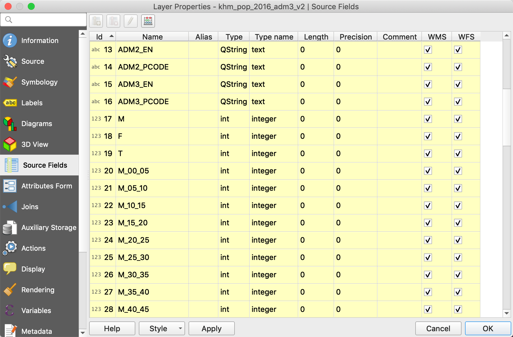
When opening this file with the Open Attribute Table button ![]() (or by right-clicking on its name), you can verify that the data attributes (M, F, T) are in a numeric format (right alignment).
(or by right-clicking on its name), you can verify that the data attributes (M, F, T) are in a numeric format (right alignment).
You can also verify the type of each attribute by opening the Layer Properties window (double-click on the name of the table) and opening the Source Fields tab.
- Open the Layer Properties window (double-click on the name of the table) of the shapefile in which you want to join the table
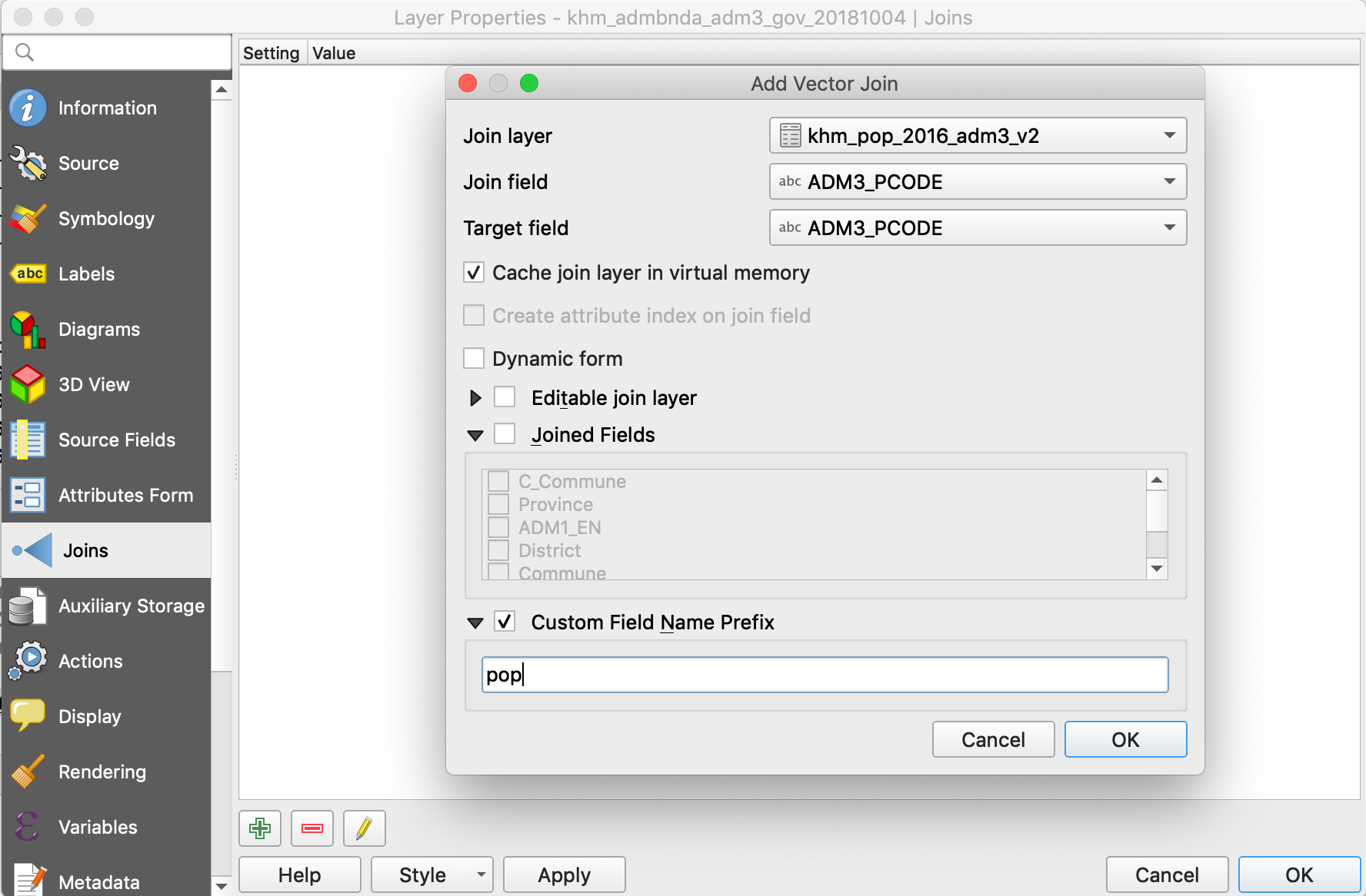
- Open the Joins tab and click on the “Add New Join” button (green + button) to add the table
- Select:
- Join layer = khm_pop_2016_adm3_v2.csv
- Join field = ADM3_PCODE
- Target field = ADM3_PCODE
- Check the “Custom Field Name Prefix” and choose a short prefix such as “pop”, otherwise the name of the joined attributes will be too long
- OK
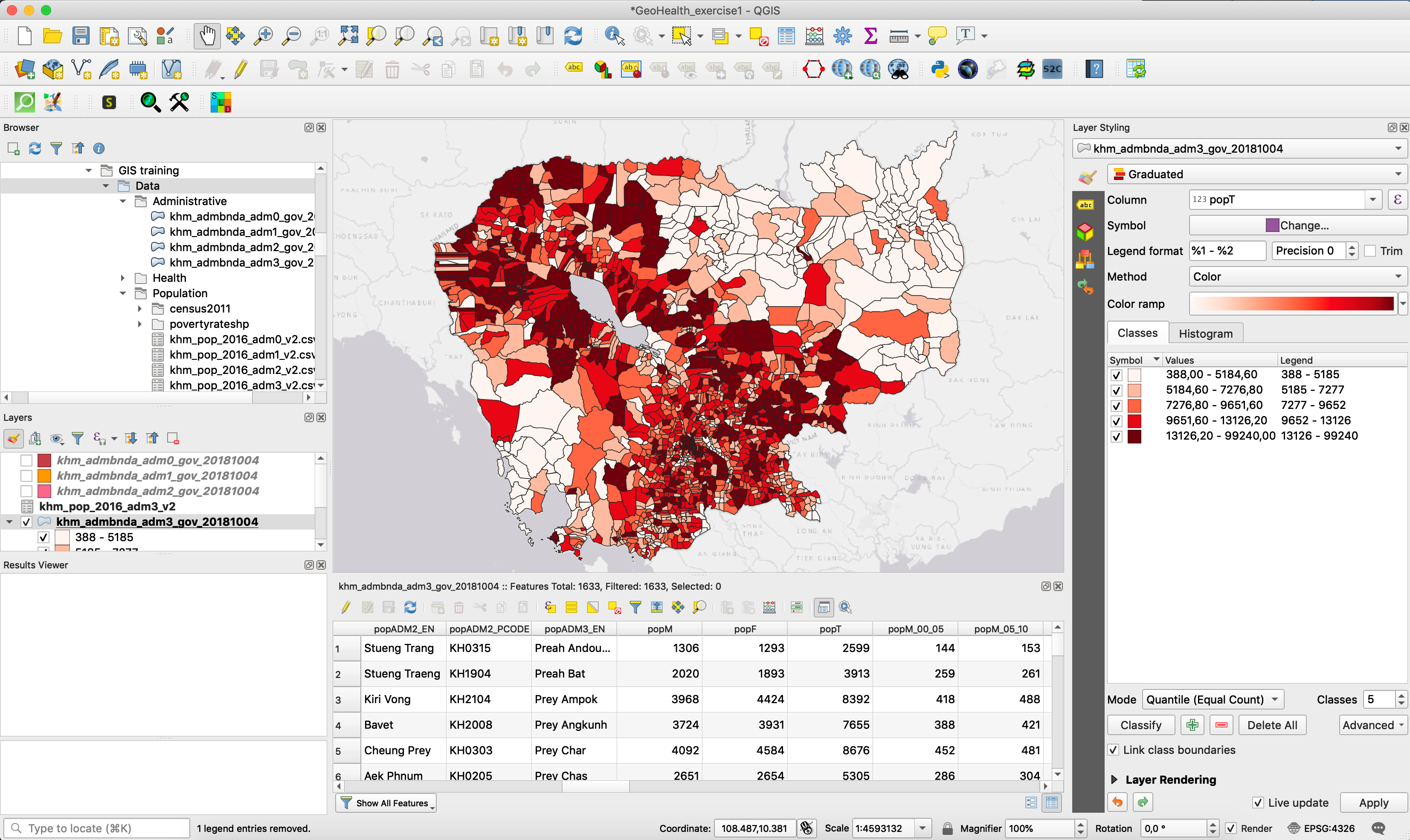
- Check that the join has enriched the attribute table of the communes layer.
- Save this new layer under a new name to permanently record the information in the attribute table
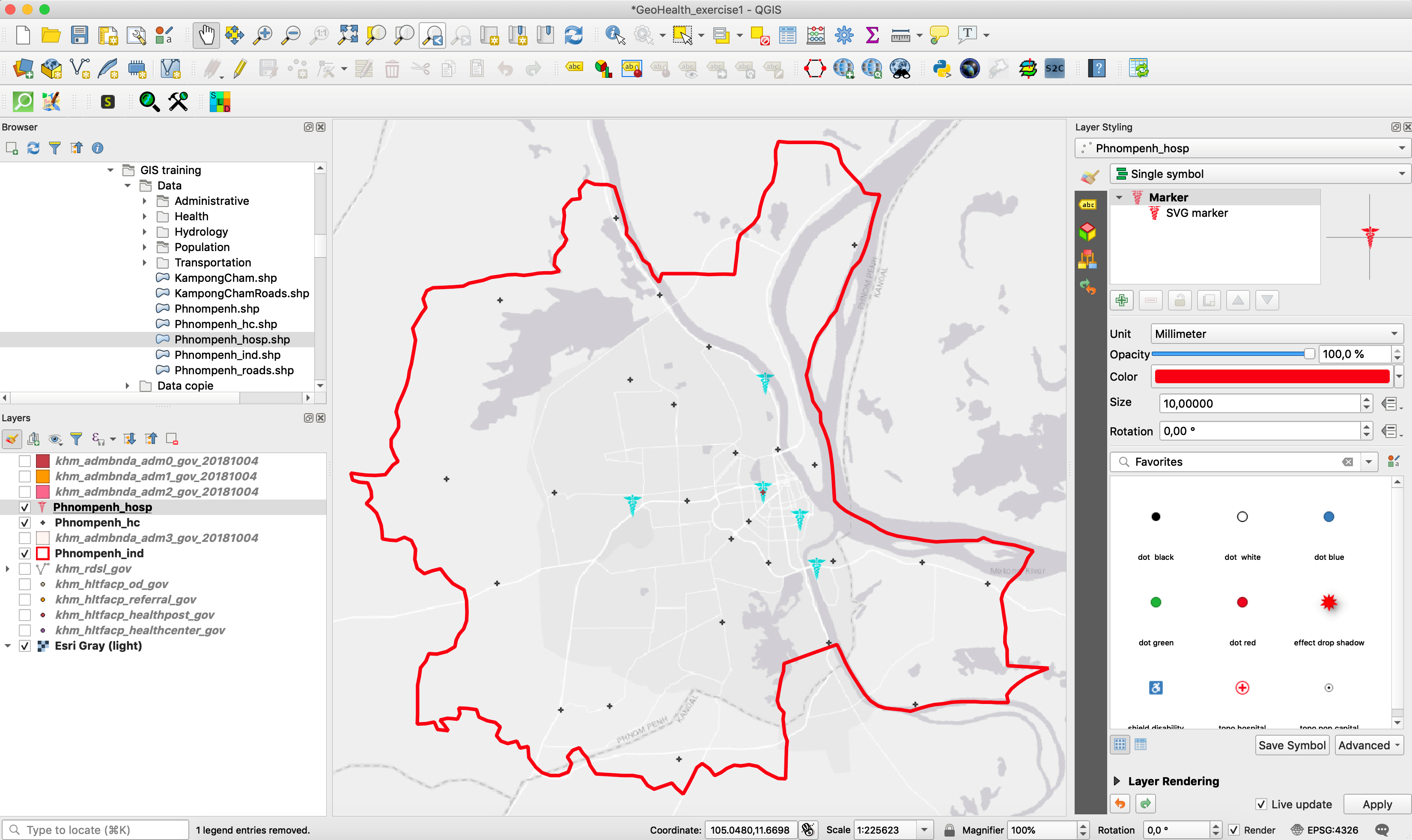
- Choose a symbology to display population data:
- Open the Layer Styling panel
- Choose “Graduated” for a continuous variable, and select the column to display
- Choose a “Color ramp”, a “Mode” (Equal Interval, Quantile, Natural Breaks, Standard Deviation, Pretty breaks) and click on “Classify”, then “Apply”
3.3 Creating new attributes in the attribute table
In this exercise, we will calculate the population densities from the Commune layer, which has been enriched with the population data per commune. It will first be necessary to the surface areas of each municipality and then divide the population by the surface area:
- Open the Attribute Table
 of the Commune layer
 - We will use the buttons above the table dedicated to editing the table:
- Open the Attribute Table

- First click on the pencil to activate the edit mode, the other buttons then become accessible.
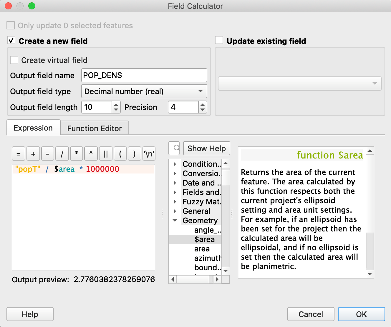
- Click on the Open Field Calculator button

- Choose create a new field for Population density as Decimal number
- Choose from the Fields and values list the attribute for Total population "popT"
- Choose the function: here in the Geometry list, double click on $area
- Write the expression: "popT" / $area * 1000000 (multiply by 1 million to have the densities in sq. km)
- The output preview shows that the calculation is indeed consistent
- Click OK
- Finally click on the Pencil button to exit the editing mode and Save.
- Note: When you switch to edit mode of the attribute table, it is also the shapefile that can be modified.
- Check consistency in the population field of the attribute table or by displaying on the map.
- Note: When you switch to edit mode of the attribute table, it is also the shapefile that can be modified.
3.4 Creating a map from a selection of entities
Exercise: Create a map of Phnom Penh Municipality (province)
- Open the province shapefile: khm_admbnda_adm1_gov_20181004.shp
- Select Phnom Penh
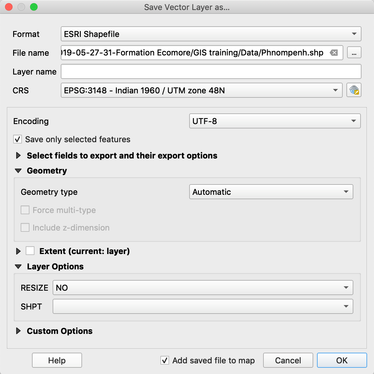
- Right click on the layer name and choose Export / Save Selected Features As…
- Choose the ESRI format, the destination of your new shapefile, name it
- OK
3.5 Intersecting vector layers
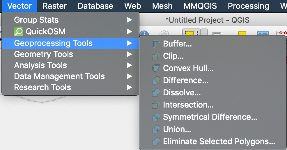
QGIS offers a set of geoprocessing tools available in the Vector menu.
Exercise: Extract health facilities in your province of interest (example of Phnom Penh)
- Add the shapefiles of the referral hospitals and of the health centers to your map canvas and check their CRS (-> Indian 60 / UTM zone 48N)
- Add the shapefile of one province (here we take Phnom Penh) and check its CRS (-> WGS 84)
- Project this shapefile into the local projected CRS
- Go to the Vector Menu / Geoprocessing tools / Intersection…
- Input layer = khm_hltfacp_referral_gov.shp
- Overlay layer = Phnompenh_ind.shp
- Intersection: browse to your folder and choose a name for the resulting intersection shapefile
- Run

3.6 Creating a layer from GPS coordinates
Exercise: Create a shapefile from a csv file containing the longitude and latitude of Phnom Penh hospitals (as referred in OpenStreetMap).
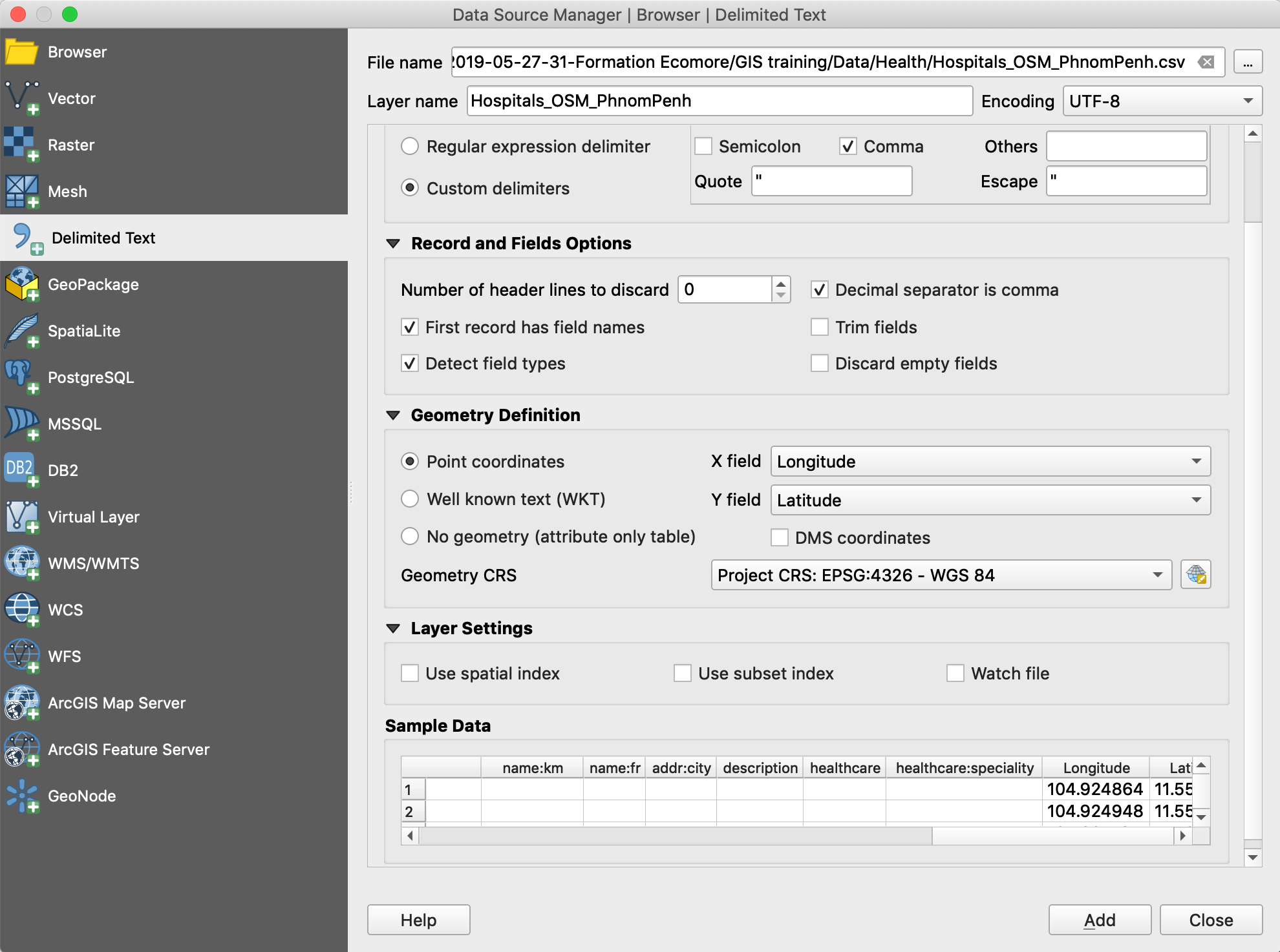
- Open the Data Source Manager
 , choose the “Delimited Text” tab and browse to your csv file: Hospitals_OSM_PhnomPenh.csv
 - Precise the file format (here, we use custom delimiters and check Comma) -> the table should be readable in the “Sample Data” box
- Precise the geometry: check “Point coordinates” and indicate the X and Y fields
- Precise the CRS of these points
- Press “Add”
- Save these imported points as a shapefile: right-click on the name of the imported file, choose Export / Save features as…
- Open the Data Source Manager
3.7 Creating buffer zones (buffers)
For the creation of buffer zones, we need a CRS in meters.
Exercise: Create buffers zones around health facilities
- Add the hospital layer to the canvas: khm_hltfacp_referral_gov.shp
- Check its CRS (-> Indian 60 / UTM zone 48N)
- Go to Vector menu / Geoprocessing Tools / Buffer…
- Choose Distance (for example here 10 kms), whether the overlapping buffers are dissolved or not, and a place to save your Buffered shapefile
- Run
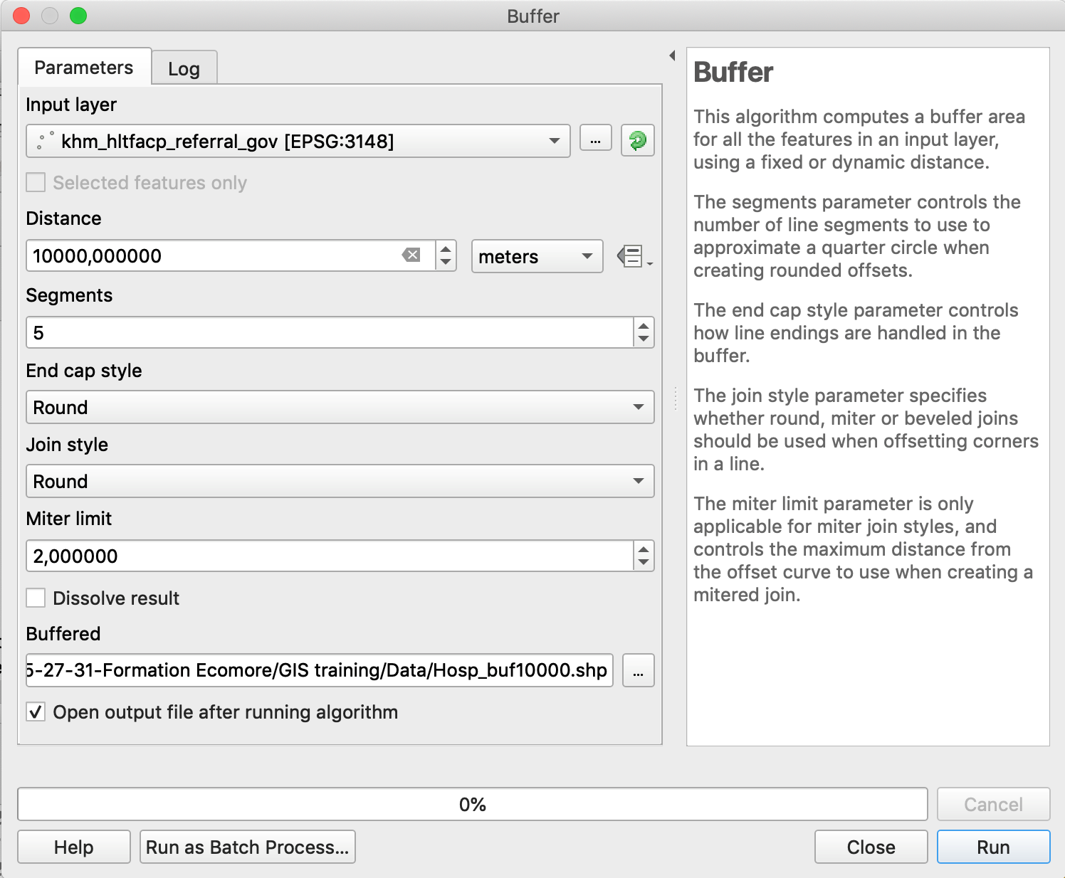
Note: Buffer zones can be created from any type of vector file (points / lines / polygons). The buffer zones will always be polygons.
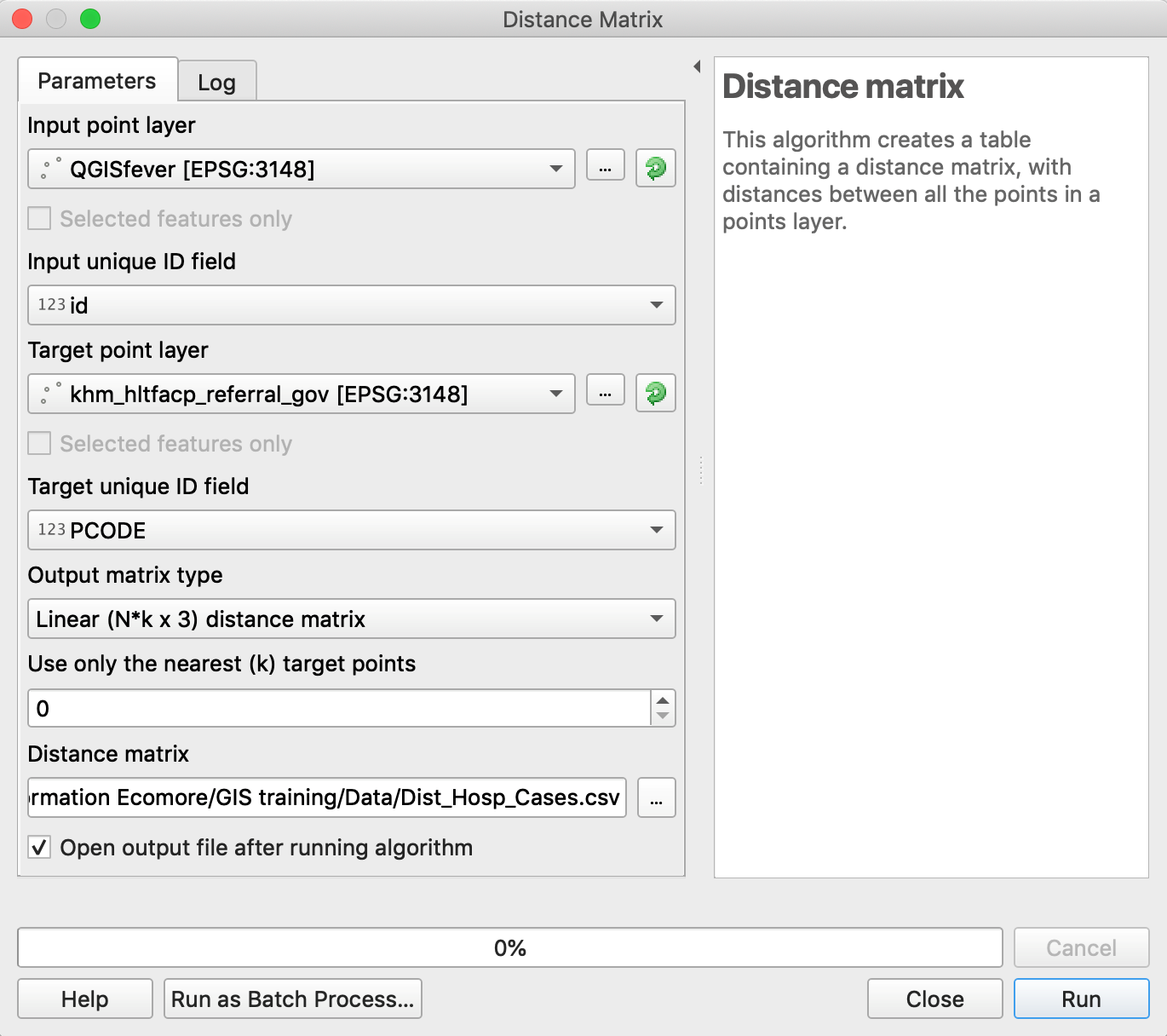
3.8 Calculating distances between points (distance matrices)
A dedicated QGIS function allows you to directly calculate distances between two layers of points.
Exercise: Calculate the distances between the locations of the fictive patients (QGISfever.shp) and referral hospitals (khm_hltfacp_referral_gov.shp).
As with the creation of buffer zones, we need a CRS in meters to calculate distances.
- Go to Vector Menu / Analysis Tools / Distance Matrix…
- Choose the two point layers (containing n cases and m infrastructures)
- Choose the type of matrix:
- Linear distance matrix where all combinations will be in line (n*m lines)
- Standard distance matrix (with n rows and m columns)
- Specify the name and location of the output distance matrix. This matrix will be in.csv format
3.9 Calculating the number of points in a polygon
This function is very useful in epidemiology for calculating, for example, the number of cases per administrative unit.
Exercise: Calculate the number of “QGIS fever” cases in each district of Phnom Penh
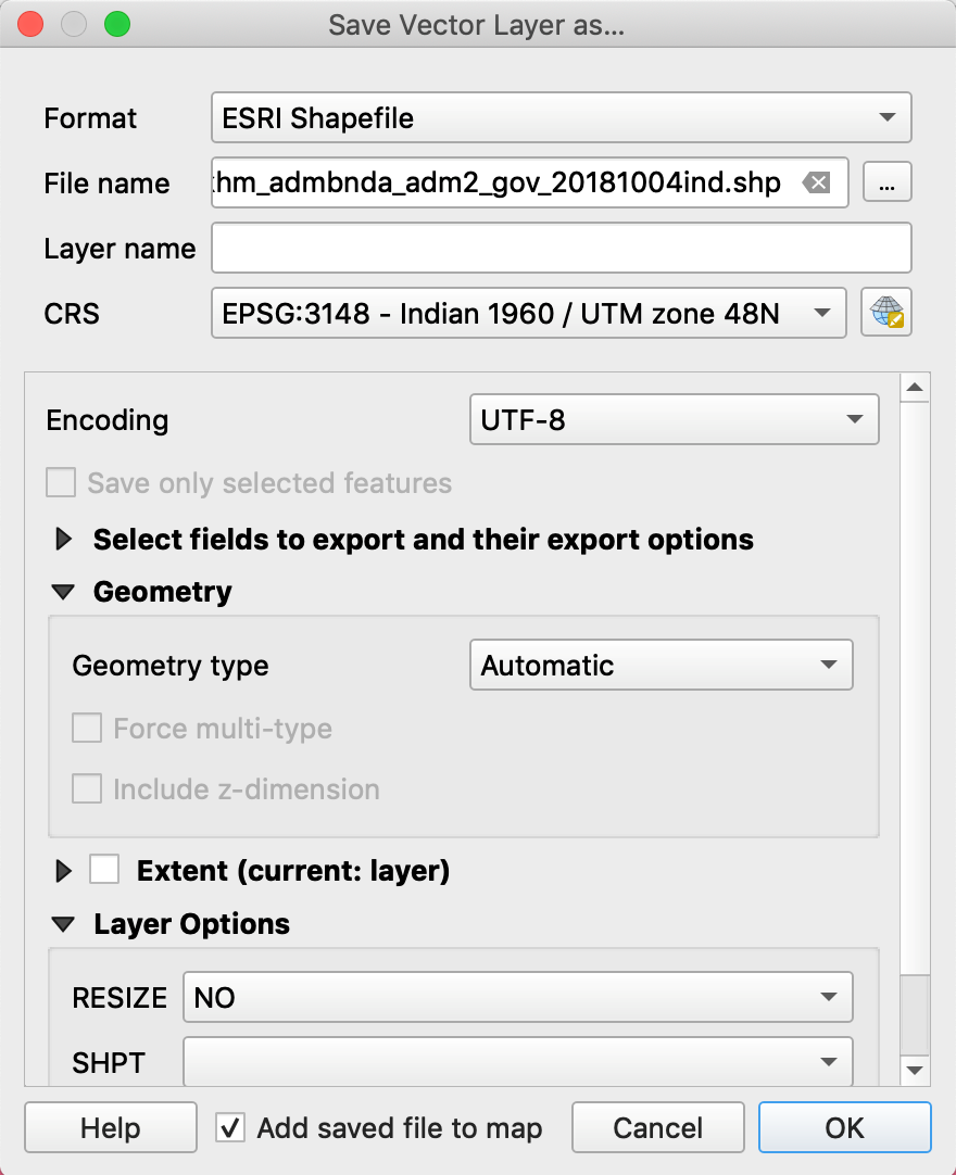
- Reproject the district layer in the local projected CRS (Indian 60 / UTM zone 48N)
- Right-click on the name of the layer
- Export / Save Features As…
- Browse to your folder and give a new name indicated they are reprojected.
- Choose the new CRS
- OK
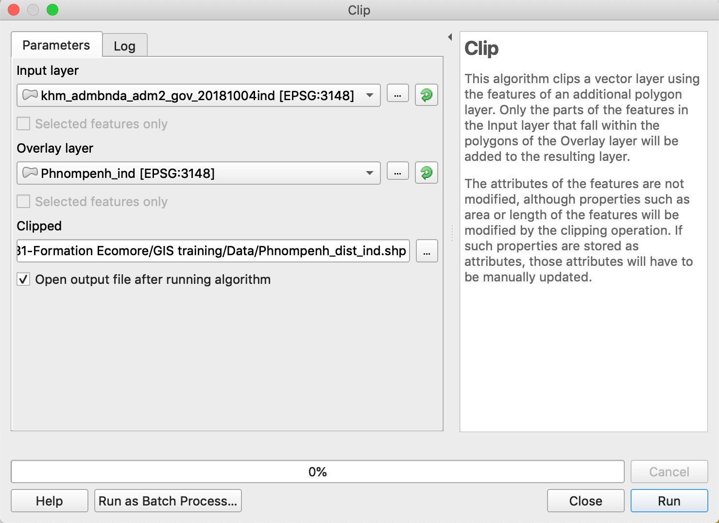
- Clip the district layer to the extent of Phnom Penh province:
- Go to Vector Menu / Geoprocessing Tools / Clip…
- Choose the district layer as the input layer
- Choose the Phnom Penh layer as the overlay layer
- Browse to your folder and give a name to the clipped layer
- Run
- Reproject the district layer in the local projected CRS (Indian 60 / UTM zone 48N)
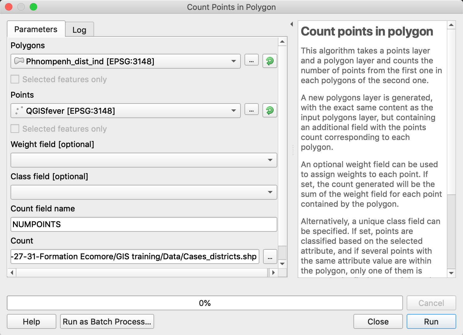
- Analysis Tools / Count Points in Polygon…
- Choose the district layer as Polygons
- Choose the QGIS fever layer as Points
- See the possible options to Weight fields (not used here)
- Specify a file name and folder for your output shapefile.
- Analysis Tools / Count Points in Polygon…
You can then represent the number of cases in each district by playing with the symbology
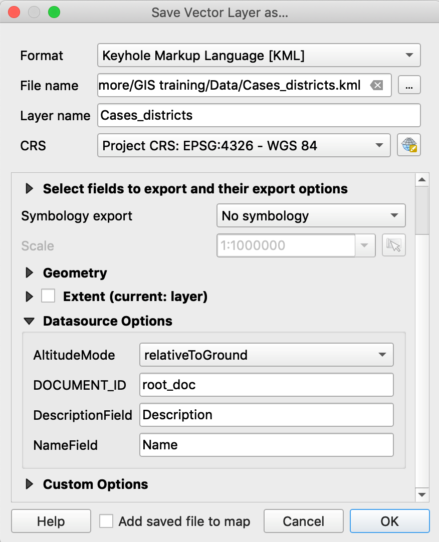
3.10 Exporting a layer to Google Earth
Note: This export could be useful when you want to exchange files with colleagues who do not know how to use a GIS, but who know the possibilities of Google Earth.
- Right-click on the name of your layer and choose Export / Save Features As…
- Choose the KML (Keyhole Markup Language) format
- Select the folder and name of your kml file to save
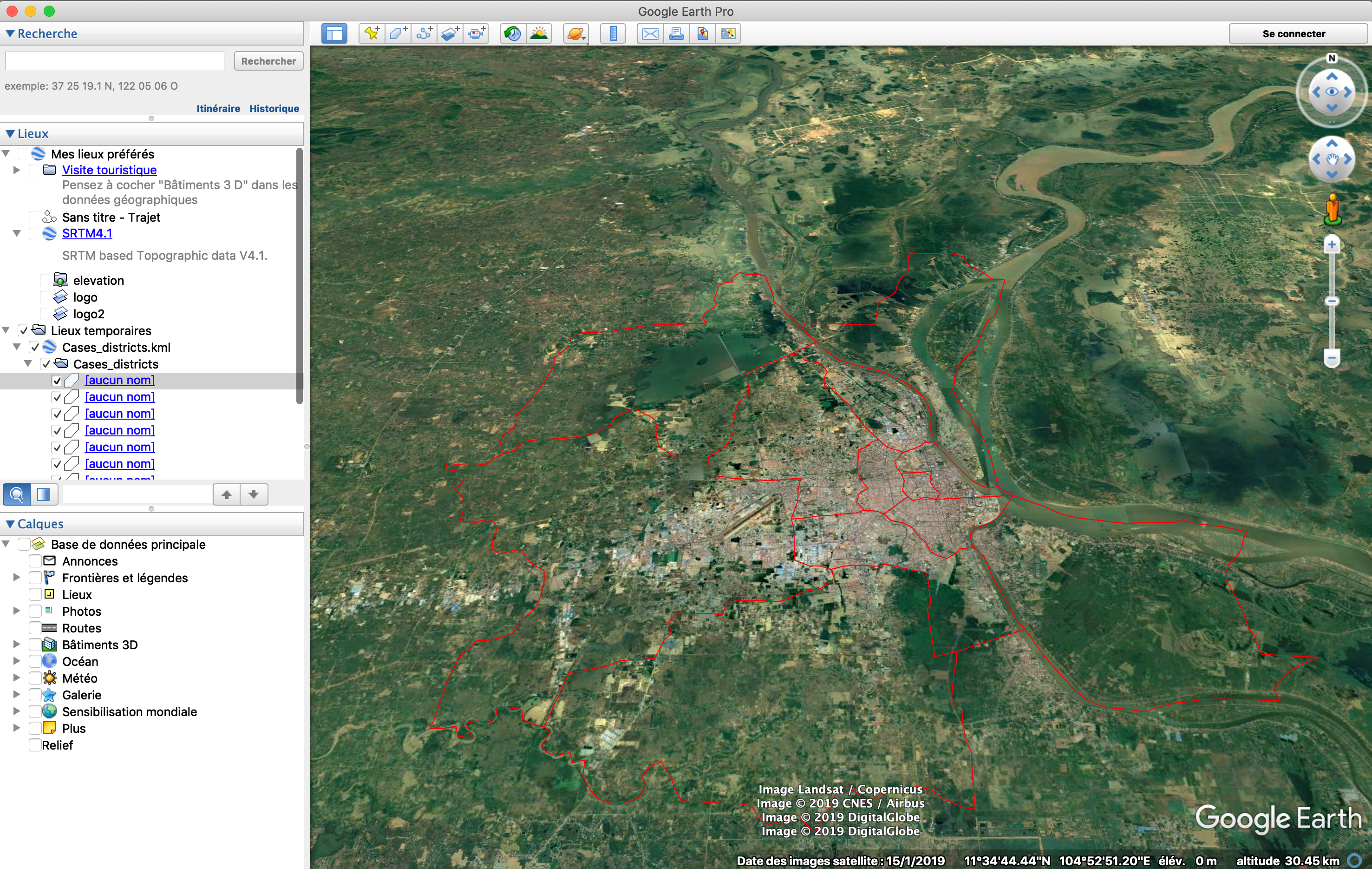
- OK
This kml file can be opened in Google Earth.